Recommendation for the Entropy Sources Used for Random Bit Generation

This Recommendation specifies the design principles and requirements for the entropy sources used by Random Bit Generators, and the tests for the validation of entropy sources. These entropy sources are intended to be combined with Deterministic Random Bit Generator mechanisms that are specified in SP 800-90A to construct Random Bit Generators, as specified in SP 800-90C.

---

---

1Introduction

1.1Scope

Cryptography and security applications make extensive use of random numbers and random bits. However, the generation of random bits is problematic in many practical applications of cryptography. The NIST Special Publication (SP) 800-90 series of Recommendations provides guidance on the construction and validation of Random Bit Generators (RBGs) in the form of Deterministic Random Bit Generators (DRBGs) (also known as pseudorandom number generators ) or Non-deterministic Random Bit Generators (NRBGs) that can be used for cryptographic applications. This Recommendation specifies how to design and test entropy sources that can be used by these RBGs. SP 800-90A addresses the construction of approved DRBG mechanisms, while SP 800-90C addresses the construction of RBGs from the mechanisms in SP 800-90A and the entropy sources in SP 800-90B. These Recommendations provide a basis for validation by NIST's Cryptographic Algorithm Validation Program (CAVP) and Cryptographic Module Validation Program (CMVP).

An entropy source that conforms to this Recommendation can be used by RBGs to produce a sequence of random bits. The outputs of entropy sources should contain a sufficient amount of randomness to provide security. This Recommendation describes the properties that an entropy source must have to make it suitable for use by cryptographic random bit generators, as well as the tests used to validate the quality of the entropy source.

The development of entropy sources that construct unpredictable outputs is difficult, and providing guidance for their design and validation testing is even more so. The testing approach defined in this Recommendation assumes that the developer understands the behavior of the source of randomness within the entropy source and has made a good-faith effort to produce an entropy source suitable for cryptographic applications (e.g., produces bitstrings that can provide entropy at a rate that meets (or exceeds) a specified value). It is expected that, over time, improvements to the guidance and testing will be made, based on experience in using and validating against this Recommendation.

This Recommendation is intended for use by entropy source developers (the entity that designs and builds the entropy source or a portion thereof), submitters11The submitter may or may not be a developer; if the submitter is not the developer then the submitter may need to acquire required information from the developer before submission or during validation testing. (the entity that submits the entropy source for validation testing), NVLAP-accredited laboratories that validate entropy sources and any entity with an interest in having an entropy source validated.1The submitter may or may not be a developer; if the submitter is not the developer then the submitter may need to acquire required information from the developer before submission or during validation testing.

This Recommendation was developed in concert with American National Standard (ANS) X9.82, a multi-part standard on random number generation.

1.2Organization

Section 2 gives a general discussion on min-entropy, the entropy source model and the conceptual interfaces. Section 3 explains the validation process and lists the requirements on the entropy source, data collection, documentation, etc. Section 4 describes the health tests. Section 5 includes various statistical tests to check whether or not the entropy source outputs are IID (independent and identically distributed). Section 6 provides several methods to estimate the entropy of the noise source. The appendices include a list of acronyms, a glossary, references, a discussion on minentropy and the optimum-guessing-attack cost, information about the narrowest internal width, Cipher Block Chaining – Message Authentication Code (CBC-MAC) specification, and the underlying information on different entropy estimation strategies used in this Recommendation.

1.3Symbols

The following symbols and functions are used in this Recommendation.

Symbol	Definition
$A=\{x_1,x_2,...,x_k\}$	The alphabet, i.e., the set of all possible symbols that a (digitized) noise source produces
$H$	The min-entropy of the samples from a (digitized) noise source or of the output from an entropy source; the min-entropy assessment for a noise source or entropy source
$H_I$	Initial entropy estimate
$H_\text{original}$	Entropy estimate of the sequential dataset
$H_\text{submitter}$	The entropy estimate provided by the submitter
$L$	The number of samples
$\log_b(x)$	The logarithm of $x$ with respect to base $b$
$\ln(x)$	The natural logarithm
$\text{min}(a, b)$	A function that returns the minimum of the two values $a$ and $b$
$\text{max}(a, b)$	A function that returns the maximum of the two values $a$ and $b$
$M[i][j]$	The $j$-th sample from the $i$-th restart of the noise source
$n$	The length of $x_i$ in bits
$nw$	Narrowest width of the conditioning component
$k$	The number of possible symbols, i.e., the size of the alphabet
$\alpha$	The probability of falsely rejecting the null hypothesis (type I error)
$|a|$	A function that returns the absolute value of $a$.
$p_i$	The probability for an observation (or occurrence) of the symbol $x_i$ in $A$.
$p_\text{max}$	The probability of observing the most common symbol from a noise source
$S = ( s_1,...,s_L )$	A dataset that consists of an ordered collection of $L$ samples, where $s_i \in A$.
$x_i$	A possible output from the (digitized) noise source.
$[a,b]$	The interval of numbers between $a$ and $b$, including $a$ and $b$.
$\lceil x \rceil$	A function that returns the smallest integer greater than or equal to $x$; also known as the ceiling function.
$\lfloor x \rfloor$	A function that returns the largest integer less than or equal to $x$; also known as the floor function.
$|$	Concatenation.
$\oplus$	Bit-wise exclusive-or operation.

2General Discussion

The three main components of a cryptographic RBG are a source of random bits (an entropy source), an algorithm for accumulating and providing random bits to the consuming applications, and a way to combine the first two components appropriately for cryptographic applications. This Recommendation describes how to design and test entropy sources. SP 800-90A describes deterministic algorithms that take an entropy input and use it to produce pseudorandom values. SP 800-90C provides the "glue" for putting the entropy source together with the algorithm to implement an RBG.

Specifying an entropy source is a complicated matter. This is partly due to confusion in the meaning of entropy, and partly due to the fact that, while other parts of an RBG design are strictly algorithmic, entropy sources depend on physical processes that may vary from one instance of a source to another. This section discusses, in detail, both the entropy source model and the meaning of entropy.

2.1Min-Entropy

The central mathematical concept underlying this Recommendation is entropy. Entropy is defined relative to one's knowledge of an experiment's output prior to observation, and reflects the uncertainty associated with predicting its value – the larger the amount of entropy, the greater the uncertainty in predicting the value of an observation. There are many possible measures for entropy; this Recommendation uses a very conservative measure known as min-entropy, which measures the effectiveness of the strategy of guessing the most likely output of the entropy source (see Appendix D and [Cac97] for more information).

In cryptography, the unpredictability of secret values (such as cryptographic keys) is essential. The probability that a secret is guessed correctly in the first trial is related to the min-entropy of the distribution that the secret was generated from.

The min-entropy of an independent discrete random variable $X$ that takes values from the set $A = \{x_1, x_2, \ldots, x_k\}$ with probability $\Pr(X = x_i) = p_i$ for $i = 1, \ldots, k$ is defined as

$$H = \min_{1 \leq i \leq k}\left(-\log_2 p_i\right) = -\log_2 \max_{1 \leq i \leq k} p_i$$

If $X$ has min-entropy $H$, then the probability of observing any particular value for $X$ is no greater than $2^{-H}$. The maximum possible value for the min-entropy of a random variable with $k$ distinct values is $\log_2 k$, which is attained when the random variable has a uniform probability distribution, i.e., $p_1 = p_2 = \cdots = p_k = 1/k$.

2.2The Entropy Source Model

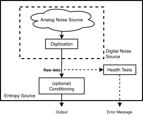
This section describes the entropy source model in detail. Figure 1 illustrates the model that this Recommendation uses to describe an entropy source and its components, which consist of a noise source, an optional conditioning component and a health testing component.

Figure 1: Entropy Source Model A block diagram of the entropy source. An analog noise source feeds a digitization step — together forming the digital noise source — which produces the raw data. The raw data is passed to an optional conditioning component that produces the entropy source output, and is also supplied to the health tests, which emit an error message on failure.

2.2.1Noise Source

The noise source is the root of security for the entropy source and for the RBG as a whole. This is the component that contains the non-deterministic, entropy-providing process that is ultimately responsible for the uncertainty associated with the bitstrings output by the entropy source.

If the non-deterministic activity being sampled produces something other than binary data, the sampling process includes a digitization process that converts the output samples to bits. The output of the digitized noise source is called the raw data.

This Recommendation assumes that the sample values (i.e., the symbols) obtained from a noise source consist of fixed-length bitstrings.

Noise sources can be divided into two categories: Physical noise sources use dedicated hardware to generate randomness; whereas Non-physical noise sources use system data (such as output of Application Programming Interface (API) functions, Random Access Memory (RAM) data or system time) or human input (e.g., mouse movements) to generate randomness.

If the noise source fails to generate random outputs, no other component in the RBG can compensate for the lack of entropy; hence, no security guarantees can be made for the application relying on the RBG.

2.2.2Conditioning Component

The optional conditioning component is a deterministic function responsible for reducing bias and/or increasing the entropy rate of the resulting output bits (if necessary to obtain a target value). There are various methods for achieving this. The developer should consider how the conditioning component to be used and how variations in the behavior of the noise source may affect the entropy rate of the output. In choosing an approach to implement, the developer may either choose to implement a cryptographic algorithm listed in Section 3.1.5.1.1 or use an alternative algorithm as a conditioning component. The use of either of these approaches is permitted by this Recommendation.

2.2.3Health Tests

Health tests are an integral part of the entropy source design that are intended to ensure that the noise source and the entire entropy source continue to operate as expected. When testing the entropy source, the end goal is to obtain assurance that failures of the entropy source are caught quickly and with a high probability. Another aspect of health testing strategy is determining the likely failure modes for the entropy source and, in particular, for the noise source. Health tests are expected to include tests that can detect these failure conditions.

The health tests can be separated into three categories: start-up tests, continuous tests (primarily on the noise source), and on-demand tests (see Section 4 for more information).

2.3Conceptual Interfaces

This section describes three conceptual interfaces that can be used to interact with the entropy source: GetEntropy, GetNoise and HealthTest. However, it is anticipated that the actual interfaces used may depend on the entropy source employed.

These interfaces can be used when constructing an RBG as specified in SP 800-90C.

2.3.1GetEntropy: An Interface to the Entropy Source

The GetEntropy interface can be considered to be a command interface into the outer entropy source box in Figure 1. This interface is meant to indicate the types of requests for services that an entropy source may support.

A GetEntropy call could return a bitstring containing the requested amount of entropy, along with an indication of the status of the request. Optionally, an assessment of the entropy can be provided. Note that the length of the returned bitstring may be greater than the amount of entropy requested.

GetEntropy

Field	Description
Input
bits_of_entropy	The requested amount of entropy.
Output
entropy_bitstring	The string that provides the requested entropy.
status	A Boolean value that is TRUE if the request has been satisfied, and FALSE otherwise.

2.3.2GetNoise: An Interface to the Noise Source

The GetNoise interface can be considered to be a command interface into the noise source component of an entropy source. This could be used to obtain raw, digitized outputs from the noise source for use in validation testing or for external health (i.e., testing performed external to the entropy source). While it is not required to be in this form, it is expected that an interface be available that allows noise source data to be obtained without harm to the entropy source. This interface is meant to provide test data to credit a noise source with an entropy estimate during validation or for external health testing. It is permitted that such an interface be available only in "test mode" and that it is disabled when the source is operational.

This interface is not intended to constrain real-world implementations, but to provide a consistent notation to describe the data collection from noise sources.

A GetNoise call returns raw, digitized samples from the noise source, along with an indication of the status of the request.

GetNoise

Field	Description
Input
number_of_samples_requested	An integer value that indicates the requested number of samples to be returned from the noise source.
Output
noise_source_data	The sequence of samples from the noise source with a length of number_of_samples_requested.
status	A Boolean value that is TRUE if the request has been satisfied, and FALSE otherwise.

2.3.3HealthTest: An Interface to the Entropy Source

A HealthTest call is a request to the entropy source to conduct a test of its health. Note that it may not be necessary to include a separate HealthTest interface if the execution of the tests can be initiated in another manner that is acceptable to FIPS 140 [FIPS140] validation.

HealthTest

Field	Description
Input
type_of_test_requested	A bitstring that indicates the type or suite of tests to be performed (this may vary from one entropy source to another).
Output
status	A Boolean value that is TRUE if the entropy source passed the requested test, and FALSE otherwise.

3Entropy Source Validation

Entropy source validation is necessary in order to obtain assurance that all relevant requirements of this Recommendation are met. This Recommendation provides requirements for validating an entropy source at a stated entropy rate. Validation consists of testing by an NVLAP-accredited laboratory against the requirements of SP 800-90B, followed by a review of the results by CAVP and CMVP. Validation provides additional assurance that adequate entropy is provided by the source and may be necessary to satisfy some legal restrictions, policies, and/or directives of various organizations.

The validation of an entropy source presents many challenges. No other part of an RBG is so dependent on the technological and environmental details of an implementation. At the same time, the proper operation of the entropy source is essential to the security of an RBG. The developer should make every effort to design an entropy source that can be shown to serve as a consistent source of entropy, producing bitstrings that can provide entropy at a rate that meets (or exceeds) a specified value. In order to design an entropy source that provides an adequate amount of entropy per output bitstring, the developer must be able to accurately estimate the amount of entropy that can be provided by sampling its (digitized) noise source. The developer must also understand the behavior of the other components included in the entropy source, since the interactions between the various components may affect any assessment of the entropy that can be provided by an implementation of the design. For example, if it is known that the raw noise-source output is biased, appropriate conditioning components can be included in the design to reduce the bias of the entropy source output to a tolerable level before any bits are output from the entropy source.

3.1Validation Process

An entropy source may be submitted to an accredited lab for validation testing by the developer or any entity with an interest in having an entropy source validated. After the entropy source is submitted for validation, the lab will examine all documentation and theoretical justifications submitted. The lab will evaluate these claims, and may ask for more evidence or clarification.

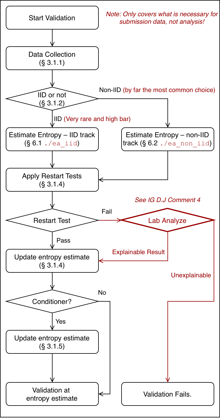
The general flow of entropy source validation testing is summarized in Figure 2. The following sections describe the details of the validation testing process.

3.1.1Data Collection

The submitter provides the following inputs for entropy estimation, according to the requirements presented in Section 3.2.4.

1. A sequential dataset of at least 1 000 000 sample values obtained directly from the noise source (i.e., raw data) shall be collected for validation22Providing additional data beyond what is required will result in more accurate entropy estimates. Lack of sufficient data may result in lower entropy estimates due to the necessity of mapping down the output values (see Section 6.4). It is recommended that, if possible, more data than is required be collected for validation. However, it is assumed in subsequent text that only the required data has been collected.. If the generation of 1 000 000 consecutive samples is not possible, the concatenation of several smaller sets of consecutive samples (generated using the same noise source) is allowed. Smaller sets shall contain at least 1000 samples. The concatenated dataset shall contain at least 1 000 000 samples.2Providing additional data beyond what is required will result in more accurate entropy estimates. Lack of sufficient data may result in lower entropy estimates due to the necessity of mapping down the output values (see Section 6.4). It is recommended that, if possible, more data than is required be collected for validation. However, it is assumed in subsequent text that only the required data has been collected.

2. If the entropy source includes a conditioning component that is not listed in Section 3.1.5.1.1, a conditioned sequential dataset of at least 1 000 000 consecutive conditioning component outputs shall be collected for validation. The output of the conditioning component shall be concatenated in the order in which it was generated and treated as a binary string for testing purposes. Note that the data collected from the noise source for validation may be used as input to the conditioning component for the collection of conditioned output values.

3. For the restart tests (see Section 3.1.4), the entropy source must be restarted 1000 times; for each restart, 1000 consecutive samples shall be collected directly from the noise source. The restart data shall be extracted whenever the noise source is ready and able to provide data that can be used for producing entropy source output. This data is stored in a 1000×1000 restart matrix $M$, where $M[i][j]$ represents the $j$-th sample from the $i$-th restart.

3.1.2Determining the track: IID track vs. non-IID track

In this Recommendation, entropy estimation is done using two different tracks: an IID-track and a non-IID track. The IID-track (see Section 6.1) is used for entropy sources that generate IID (independent and identically distributed) samples, whereas the non-IID track (see Section 6.2) is used for noise sources that do not generate IID samples.

The track selection is done based on the following rules. The IID track shall be used only when all of the following conditions are satisfied:

1. The submitter makes an IID claim on the noise source, based on the submitter's analysis of the design. The submitter shall provide rationale for the IID claim.

2. The sequential dataset described in item 1 of Section 3.1.1 is tested using the statistical tests described in Section 5 to verify the IID assumption, and the IID assumption is verified (i.e., there is no evidence that the data is not IID).

3. The row and column datasets described in item 3 of Section 3.1.1 are tested using the statistical tests described in Section 5 to verify the IID assumption, and the IID assumption is verified.

4. If a conditioning component that is not listed in Section 3.1.5.1.1 is used, the conditioned sequential dataset (described in item 2 of Section 3.1.1) is tested using the statistical tests described in Section 5 to verify the IID assumption, and the IID assumption is verified.

If any of these conditions are not met, the estimation process shall follow the non-IID track.

3.1.3Initial Entropy Estimate

The submitter shall provide an entropy estimate for the noise source outputs, which is based on the submitter's analysis of the noise source (see Requirement 3 in Section 3.2.2). This estimate is denoted as $H_{submitter}$.

After determining the entropy estimation track, a min-entropy estimate per sample, denoted as $H_{original}$, for the sequential dataset is calculated using the methods described in Section 6.1 (for the IID track) or Section 6.2 (for the non-IID track). If the alphabet size is greater than 256, it shall be reduced to at most 256 symbols (see Section 6.4).

If the sequential dataset is not binary, an additional entropy estimation (per bit), denoted $H_{bitstring}$, is estimated. First, the sequential dataset that contains $L$ samples (each having $n$ bits) is considered as a bitstring of size $nL$. The bits after the first 1 000 000 bits may be ignored. Then, the estimation is done based on the entropy estimation track, as specified in the previous paragraph, and $H_{bitstring}$ is calculated. Then, the entropy per sample is estimated to be $n \times H_{bitstring}$.

The initial entropy estimate of the noise source is calculated as $H_I = \min(H_{original}, n \times H_{bitstring}, H_{submitter})$ for non-binary sources and as $H_I = \min(H_{original}, H_{submitter})$ for binary sources.

3.1.4Restart Tests

The entropy estimate of a noise source, calculated from a single, long-output sequence, might provide an overestimate if the noise source generates correlated sequences after restarts. Hence, an attacker with access to multiple noise source output sequences after restarts may be able to predict the next output sequence with much better success than the entropy estimate suggests.

The process of restarting a noise source may be different for different noise sources (e.g., powering off, cooling off, delaying ten seconds before extracting output from the noise source, etc.). The submitter shall define the restart process suitable for the submission. This process shall simulate the restart process expected in real-world use (e.g., the outputs are not generated until after the start-up tests are complete; see Section 4.2). All restarts are expected to be done in normal operating conditions.

The restart tests described in this section re-evaluate the entropy estimate for the noise source using different outputs from many restarts of the noise source. These tests are designed to ensure that:

• The noise source outputs generated after a restart are drawn from the same distribution as every other output.
• The distribution of samples in a restart sequence is independent of its position in the restart sequence.
• The knowledge of other restart sequences does not offer additional advantage in predicting the next restart sequence.

3.1.4.1Constructing Restart Data

To construct restart data, the entropy source shall be restarted $r = 1000$ times; for each restart, $c = 1000$ consecutive samples shall be collected directly from the noise source. The collection of the data shall be done as soon as the entropy source is ready to produce outputs for real-world use (e.g., after start-up tests). Note that an entropy source, in its real-world use and during restart testing, may inhibit outputs for a time immediately after restarting in order to allow any transient weak behavior to pass. The output samples are stored in an $r$ by $c$ matrix $M$, where $M[i][j]$ represents the $j$-th sample from the $i$-th restart.

Two datasets are constructed using the matrix $M$:

• The row dataset is constructed by concatenating the rows of the matrix $M$, i.e., the row dataset is $M[1][1] \,\|\, \ldots \,\|\, M[1][c] \,\|\, M[2][1] \,\|\, \ldots \,\|\, M[2][c] \,\|\, \ldots \,\|\, M[r][1] \,\|\, \ldots \,\|\, M[r][c]$.
• The column dataset is constructed by concatenating the columns of the matrix $M$, i.e., the column dataset is $M[1][1] \,\|\, \ldots \,\|\, M[r][1] \,\|\, M[1][2] \,\|\, \ldots \,\|\, M[r][2] \,\|\, \ldots \,\|\, M[1][c] \,\|\, \ldots \,\|\, M[r][c]$.

3.1.4.2Validation Testing

The restart tests check the relations between noise source samples generated after restarting the entropy source, and compare the results to the initial entropy estimate, $H_I$ (see Section 3.1.3).

First, the sanity check described in Section 3.1.4.3 is performed on the matrix $M$. If the test fails, the validation fails and no entropy estimate is awarded.

If the noise source does not fail the sanity check, then the entropy estimation methods described in Section 6.1 (for the IID track) or Section 6.2 (for the non-IID track) are performed on the row and the column datasets, based on the track of the entropy source. Let $H_r$ and $H_c$ be the resulting entropy estimates of the row and the column datasets, respectively. The entropy estimates from the row and the column datasets are expected to be close to the initial entropy estimate $H_I$. If the minimum of $H_r$ and $H_c$ is less than half of $H_I$, the validation fails, and no entropy estimate is awarded. Otherwise, the entropy assessment of the noise source is taken as the minimum of the row, the column and the initial estimates, i.e., $\min(H_r, H_c, H_I)$.

If the noise source does not fail the restart tests, and the entropy source does not include a conditioning component, the entropy source will be validated at $H = \min(H_r, H_c, H_I)$. If the entropy source includes a conditioning component, the entropy assessment of the entropy source is updated as described in Section 3.1.5.

3.1.4.3Sanity Check - Most Common Value in the Rows and Columns

This test checks the frequency of the most common value in the rows and the columns of the matrix $M$. If this frequency is significantly greater than the expected value, given the initial entropy estimate $H_I$ calculated in Section 3.1.3, the restart test fails. In this case, the validation fails no entropy estimate is awarded.

This sanity check is based on a binomial test, where there are two possible outcomes for each trial: the most frequent value or any other value is observed. The purpose of the test is to determine whether the most frequent value appears more than would be expected, given the initial entropy estimate, $H_I$. The probability of type I error, denoted $\alpha$, is set at 0.01 over the entire sanity check, where each of the 2000 binomial experiments33The experiments done for each row or column are considered to be independent. has type I error probability of 0.000 005.3The experiments done for each row or column are considered to be independent.

Only the experiment yielding the highest count is tested. If that experiment passes the test, then the other 1999 experiments will pass as well. If any of the 2000 experiments were to fail, one of the failed experiments would be the experiment having the highest count. Therefore, it is sufficient to test the experiment with the highest count.

Given the 1000 by 1000 restart matrix and the initial entropy estimate $H_I$, the test is performed as follows:

1. Let $p = 2^{-H_I}$. Let $\alpha$ be 0.000 005.

2. For each row ($1 \leq i \leq 1000$) of the matrix, count the number of occurrences of each sample present in the row. Set $X_{Ri}$ to the highest count value for row $i$. Let $X_R$ be the maximum count value for all the rows, i.e., $X_R = \max(X_{R1}, \ldots, X_{R1000})$.

3. For each column ($1 \leq i \leq 1000$) of the matrix, count the number of occurrences of each sample present in the column. Set $X_{Ci}$ to the highest count value for column $i$. Let $X_C$ be the maximum count value for all the columns, i.e., $X_C = \max(X_{C1}, \ldots, X_{C1000})$.

4. Let $X_{max} = \max(X_C, X_R)$.

5. Calculate $\Pr(X \geq X_{max}) = \sum_{j=X_{max}}^{1000} \binom{1000}{j} p^j (1-p)^{1000-j}$. If $\Pr(X \geq X_{max}) < \alpha$, the test fails. Otherwise, the test passes.

3.1.5Entropy Estimation for Entropy Sources Using a Conditioning Component

The optional conditioning component gets inputs from the noise source and generates the output of the entropy source. The size of the input and the output of the conditioning component in bits, denoted as $n_{in}$ and $n_{out}$, respectively, shall be fixed and shall be specified by the submitter. Noise source outputs are concatenated to construct the $n_{in}$-bit input to the conditioning function. The entropy of the input, denoted $h_{in}$, depends on the number of samples needed to construct the $n_{in}$-bit input. If $w$ samples are needed, then $h_{in}$ is estimated to be $w \times h$ bits. The size of the conditioning component input shall be a multiple of the size of the noise source output.

Since the conditioning component is deterministic, the entropy of the output is at most $h_{in}$. However, the conditioning component may reduce the entropy of the output. The entropy of the output from the conditioning component is denoted as $h_{out}$, i.e., $h_{out}$ bits of entropy are contained within the $n_{out}$-bit output. The entropy of the output also depends on the internals of the conditioning components. In this Recommendation, the narrowest internal width within the conditioning component is denoted as $nw$. A discussion on the narrowest internal width is given in Appendix E.

Figure 3: Entropy of the Conditioning Component A block diagram. The noise source provides an input of $n_{in}$ bits carrying $h_{in}$ bits of entropy to the conditioning component (whose narrowest internal width is $nw$), which produces an output of $n_{out}$ bits carrying $h_{out}$ bits of entropy.

The optional conditioning component can be designed in various ways. Section 3.1.5.1.1 provides a list of vetted cryptographic algorithms/functions for conditioning the noise source outputs. Submitters are allowed to use other conditioning components. If a conditioning component from Section 3.1.5.1.1 is used, the entropy estimation is performed as described in Section 3.1.5.1.2; if a non-listed algorithm is used, the entropy estimation is performed as described in Section 3.1.5.2.

3.1.5.1Using Vetted Conditioning Components

Both keyed and unkeyed algorithms have been vetted for conditioning. Section 3.1.5.1.1 provides a list of vetted conditioning components. Section 3.1.5.1.2 discusses the method for determining the entropy provided by a vetted conditioning component.

List of Vetted Conditioning Components

Three keyed algorithms have been vetted for a keyed conditioning component:

1. HMAC, as specified in FIPS 198, with any approved hash function specified in FIPS 180 or FIPS 202,

2. CMAC, as specified in SP 800-38B, with the AES block cipher (see FIPS 197), and

3. CBC-MAC, as specified in Appendix F, with the AES block cipher. This Recommendation does not approve the use of CBC-MAC for purposes other than as a conditioning component in an RBG.

   Three unkeyed functions have been vetted for an unkeyed conditioning component:

4. Any approved hash function specified in FIPS 180 or FIPS 202,

5. Hash_df, as specified in SP 800-90A, using any approved hash function specified in FIPS 180 or FIPS 202, and

6. Block_Cipher_df, as specified in SP 800-90A using the AES block cipher (see FIPS 197).

The narrowest internal width and the output length for the vetted conditioning functions are provided in the following table.

Table 1: The narrowest internal width and output lengths of the vetted conditioning functions.

Conditioning Function	Narrowest Internal Width ($nw$)	Output Length ($n_{out}$)
HMAC	hash-function output size	hash-function output size
CMAC	AES block size = 128	AES block size = 128
CBC-MAC	AES block size = 128	AES block size = 128
Hash Function	hash-function output size	hash-function output size
Hash_df	hash-function output size	hash-function output size
Block_Cipher_df	AES key size	AES key size

For Hash_df and Block_Cipher_df, the output length indicated in the table is used as the no_of_bits_to_return input parameter for the invocation of Hash_df and Block_Cipher_df (see SP 800-90A).

Entropy Assessment using Vetted Conditioning Components

When using a conditioning component listed in Section 3.1.5.1.1 (given the assurance of correct implementation by CAVP testing), the entropy of the output is estimated as

$$h_{out} = \text{Output\_Entropy}(n_{in}, n_{out}, nw, h_{in})$$

where $\text{Output\_Entropy}(n_{in}, n_{out}, nw, h_{in})$ is described as follows44The formula used to generate Output_Entropy() is adapted from the formula $k_\alpha = \frac{m}{n} + \alpha\sqrt{2\frac{m}{n}\ln n}$ provided in Theorem 1 of [RaSt98], such that $m$ is equal to $2^{n_{in}}$, $n$ is equal to $2^n$ and $\alpha$ is equal to 1.:4The formula used to generate Output_Entropy() is adapted from the formula $k_\alpha = \frac{m}{n} + \alpha\sqrt{2\frac{m}{n}\ln n}$ provided in Theorem 1 of [RaSt98], such that $m$ is equal to $2^{n_{in}}$, $n$ is equal to $2^n$ and $\alpha$ is equal to 1.

1. Let $P_{high} = 2^{-h_{in}}$ and $P_{low} = \frac{1 - P_{high}}{2^{n_{in}} - 1}$.
2. $n = \min(n_{out}, nw)$.
3. $\psi = 2^{n_{in} - n} P_{low} + P_{high}$.
4. $U = 2^{n_{in} - n} + \sqrt{2n\left(2^{n_{in} - n}\right)\ln(2)}$.
5. $\omega = U \times P_{low}$.
6. Return $-\log_2\left(\max(\psi, \omega)\right)$.

The entropy source will be assessed at the min-entropy per conditioned output, $h_{out}$, computed above. Vetted conditioning components are permitted to claim full entropy outputs.

Note that it is acceptable to truncate the outputs from a vetted conditioning component. If this is done, the entropy estimate is reduced to a proportion of the output (e.g., if there are six bits of entropy in an eight-bit output and the output is truncated to six bits, then the entropy is reduced to $3/4 \times 6 = 4.5$ bits).

When additional noise sources are available, the length of the input ($n_{in}$) shall only include the inputs from the primary noise source.

3.1.5.2Using Non-vetted Conditioning Components

For non-vetted conditioning components, the entropy in the output depends on the entropy and size of the input ($h_{in}$ and $n_{in}$), the size of the output ($n_{out}$), and the size of the narrowest internal width ($nw$) and the entropy of the conditioned sequential dataset (as described in item 2 of Section 3.1.1), which shall be computed using the methods described in either Section 6.1 (for IID data) or Section 6.2 (for non-IID data). Let the obtained entropy estimate per bit be $h'$.

The output of the conditioning component ($n_{out}$) shall be treated as a binary string, for purposes of the entropy estimation.

The entropy of the conditioned output is estimated as

$$h_{out} = \min\left(\text{Output\_Entropy}(n_{in}, n_{out}, nw, h_{in}),\; 0.999\,n_{out},\; h' \times n_{out}\right).$$

The description of Output_Entropy is given in Section 3.1.5.1.2. To avoid approving an entropy source having a non-vetted conditioning component with full entropy, $n_{out}$ is multiplied by the constant 0.999. The entropy source will be validated at the min-entropy per conditioned output, $h_{out}$, computed above.

Note that truncating subsequent to the use of a non-vetted conditioning component shall not be performed before providing output from the entropy source.

3.1.6Additional Noise Sources

In this Recommendation, it is assumed that the entropy sources have a unique primary noise source that is responsible to generate randomness. It should be noted that multiple copies of the same physical noise source are considered as a single noise source (e.g., a source with eight ring oscillators, where the sampled bits are concatenated to get an eight-bit output, or where the samples bits are XORed together).

In addition to the primary noise source outputs, outputs of other noise sources may be available to the entropy source, and their outputs may be used to increase security. However, the joint entropy of these outputs may be hard to estimate, especially when there are dependencies between the sources (e.g., packet arrival times in a communication network and hard drive access times).

This Recommendation allows one to concatenate the outputs of the additional noise sources to the primary noise source to generate input to the conditioning component. In such cases, vetted conditioning components shall be used. No entropy is credited from the outputs of the additional noise sources.

3.2Requirements for Validation Testing

In this section, high-level requirements (on both submitters and testers) are presented for validation testing.

3.2.1Requirements on the Entropy Source

The intent of these requirements is to assist the developer in designing/implementing an entropy source that can provide outputs with a consistent amount of entropy and to produce the required documentation for entropy source validation.

1. The entire design of the entropy source shall be documented, including the interaction of the components specified in Section 2.2. The documentation shall justify why the entropy source can be relied upon to produce bits with entropy.

2. Documentation shall describe the operation of the entropy source, including how the entropy source works, and how to obtain data from within the entropy source for validation testing.

3. Documentation shall describe the range of operating conditions (e.g., temperature range, voltages, system activity, etc.) under which the entropy source is claimed to operate correctly. The entropy source outputs are expected to have similar entropy rates in this specified range of operating conditions.

4. The entropy source shall have a well-defined (conceptual) security boundary. This security boundary shall be documented; the documentation shall include a description of the content of the security boundary.

5. When a conditioning component is not used, the output from the entropy source is the output of the noise source, and no additional interface is required. In this case, the noise-source output is available during both validation testing and normal operation. When a conditioning component is included in the entropy source, the output from the entropy source is the output of the conditioning component, and an additional interface is required to access the noise-source output. In this case, the noise-source output shall be accessible via the interface during validation testing, but the interface may be disabled otherwise. The designer shall fully document the method used to get access to the raw noise source samples. If the noise-source interface is not disabled during normal operation, any noise-source output using this interface shall not be provided to the conditioning component for processing and eventual output as normal entropy-source output.

6. The entropy source may restrict access to raw noise source samples to special circumstances that are not available to users in the field, and the documentation shall explain why this restriction is not expected to substantially alter the behavior of the entropy source as tested during validation.

7. Documentation shall contain a description of the restarting process applied during the restart tests.

3.2.2Requirements on the Noise Source

The entropy source will have no more entropy than that provided by the noise source, and as such, the noise source requires special attention during validation testing. This is partly due to the fundamental importance of the noise source (if it does not do its job, the entropy source will not provide the expected amount of security), and partly because the probabilistic nature of its behavior requires more complicated testing.

The requirements for the noise source are as follows:

1. The operation of the noise source shall be documented; this documentation shall include a description of how the noise source works, where the unpredictability comes from, and rationale for why the noise source provides acceptable entropy output, and should reference relevant, existing research and literature.

2. The behavior of the noise source shall be stationary (i.e., the probability distributions of the noise source outputs do not change when shifted in time). Documentation shall include why it is believed that the entropy rate does not change significantly during normal operation. This can be in broad terms of where the unpredictability comes from and a rough description of the behavior of the noise source (to show that it is reasonable to assume that the behavior is stationary).

3. Documentation shall provide an explicit statement of the expected entropy provided by the noise source outputs and provide a technical argument for why the noise source can support that entropy rate. To support this, documentation may include a stochastic model of the noise source outputs, and an entropy estimation based on this stochastic model may be included.

4. The noise source state shall be protected from adversarial knowledge or influence to the greatest extent possible. The methods used for this shall be documented, including a description of the (conceptual) security boundary's role in protecting the noise source from adversarial observation or influence.

5. Although the noise source is not required to produce unbiased and independent outputs, it shall exhibit random behavior; i.e., the output shall not be definable by any known algorithmic rule. Documentation shall indicate whether the noise source produces IID data or non-IID data. This claim will be used in determining the test path followed during validation. If the submitter makes an IID claim, documentation shall include rationale for the claim.

6. The noise source shall generate fixed-length bitstrings. A description of the output space of the noise source shall be provided. Documentation shall specify the fixed symbol size (in bits) and the list (or range) of all possible outputs from each noise source.

7. If additional noise source outputs to increase security are used, a document that describes the additional noise sources shall be included.

3.2.3Requirements on the Conditioning Component

The requirements for the conditioning component are as follows:

1. The submitter shall document which conditioning component is used and the details about its implementation (e.g., the hash function and/or key size used). Documentation shall include the input and the output sizes ($n_{in}$ and $n_{out}$).

2. If the entropy source uses a vetted conditioning component as listed in Section 3.1.5.1.1, the implementation of the component shall be tested to obtain assurance of correctness before subsequent testing of the entropy source. The submitter shall specify any keys used to test the correctness of the conditioning component implementation during validation testing. If the testing fails, validation of the entropy source fails. The submitter may retest with the corrected implementation until the conditioning component passes the validation test.

3. If the conditioning component uses cryptographic keys, the keys may be (1) fixed to a predetermined value, (2) set using some additional input to the device, or (3) generated by using the noise source outputs. The key shall be determined before any outputs are generated from the conditioning component.

4. Any value which is used to determine the key shall not be used as any other input to the conditioning component. The input entropy to the conditioning component ($h_{in}$) shall not include any entropy provided to the key of a keyed function.

5. For entropy sources containing a conditioning component that is not listed in Section 3.1.5.1.1, a description of the conditioning component shall be provided. Documentation shall state the narrowest internal width and the size of the output blocks from the conditioning component. The submitter shall provide mathematical evidence that the component is suitable to be used to condition the noise source output, and does not significantly reduce the entropy rate of the entropy source output. The submitter shall also provide a justification about why the conditioning component does not act poorly when the noise source data is not independent.

3.2.4Requirements on Data Collection

The requirements on data collection are listed below:

1. The data collection for entropy estimation shall be performed in one of the three ways described below:

   • By the submitter with a witness from the testing lab, or
   • By the testing lab itself, or
   • Prepared by the submitter in advance of testing, along with the following documentation: a specification of the data generation process, and a signed document that attests that the specification was followed.

2. Data collected from the noise source for validation testing shall be raw output values.

3. The data collection process shall not require a detailed knowledge of the noise source or intrusive actions that may alter the behavior of the noise source (e.g., drilling into the device).

4. Data shall be collected from the noise source and any conditioning component that is not listed in Section 3.1.5.1.1 (if used) under normal operating conditions.

5. Data shall be collected from the entropy source under validation. Any relevant version of the hardware or software updates shall be associated with the data.

6. Documentation of the data collection method shall be provided so that a lab or submitter can perform (or replicate) the collection process at a later time, if necessary.

7. Documentation explaining why the data collection method does not interfere with the noise source shall be provided.

4Health Tests

Health tests are an important component of the entropy source, as they aim to detect deviations from the intended behavior of the noise source as quickly as possible and with a high probability. Noise sources can be fragile, and hence, can be affected by changes in the operating conditions of the device, such as the temperature, humidity, or electric field, which might result in unexpected behavior. The health tests take the entropy assessment as input55The submitter may claim a low entropy estimate (as described in Section 3.1.3) to reduce the false positive rates., and characterize the expected behavior of the noise source based on this value. Requirements on the health tests are listed in Section 4.3.5The submitter may claim a low entropy estimate (as described in Section 3.1.3) to reduce the false positive rates.

4.1Health Test Overview

The health testing of a noise source is likely to be very technology-specific. Since, in most cases, the noise source will not produce unbiased, independent binary data, traditional statistical procedures (e.g., the randomness tests described in NIST SP 800-22) that test the hypothesis of unbiased, independent bits will almost always fail, and thus are not useful for monitoring the noise source. In general, tests on the noise source need to be tailored carefully, taking into account the expected statistical behavior of the correctly operating noise source.

The health testing of noise sources will typically be designed to detect failures of the noise source, based on the expected output during a failure, or to detect a deviation from the expected output during the correct operation of the noise source. Health tests are expected to raise an alarm in three cases:

1. When there is a significant decrease in the entropy of the outputs,

2. When noise source failures occur, or

3. When hardware fails, and implementations do not work correctly.

4.2Types of Health Tests

Health tests are applied to the outputs of a noise source before any conditioning is done. (It is permissible to also apply some health tests to conditioned outputs, but this is not required.)

Start-up health tests are designed to be performed after powering up, or rebooting, and before the first use of the entropy source. They provide some assurance that the entropy source components are working as expected before they are used during normal operating conditions, and that nothing has failed since the last time that the start-up tests were run.66The specific conditions in which the startup tests must be run for FIPS-validated cryptographic modules are determined by the requirements of FIPS 140. This document imposes no additional requirements for the use of start-up health testing. The samples drawn from the noise source during the startup tests shall not be available for normal operations until the tests are completed; these samples may be discarded at any time, or may be used after the completion of the tests if there are no errors.6The specific conditions in which the startup tests must be run for FIPS-validated cryptographic modules are determined by the requirements of FIPS 140. This document imposes no additional requirements for the use of start-up health testing.

Continuous health tests are run indefinitely on the outputs of the noise source77Entropy sources may have a warm-up phase in which the outputs are inhibited for a time immediately after startup. Continuous health testing is not required during the warm up phase. while the noise source is operating. Continuous tests focus on the noise source behavior and aim to detect failures as the noise source produces outputs. The purpose of continuous tests is to allow the entropy source to detect many kinds of failures in its underlying noise source. These tests are run continuously on all digitized samples obtained from the noise source, and so tests must have a very low probability of raising a false alarm during the normal operation of the noise source. In many systems, a reasonable false positive probability will make it extremely unlikely that a properly functioning device will indicate a malfunction, even in a very long service life. Continuous tests are resource-constrained – this limits their ability to detect noise source failures so they are usually designed so that only gross failures are likely to be detected.7Entropy sources may have a warm-up phase in which the outputs are inhibited for a time immediately after startup. Continuous health testing is not required during the warm up phase.

Note that continuous health tests operate over a stream of values. These sample values may be output from the entropy source as they are generated and (optionally) processed by a conditioning component; there is no need to inhibit output from the noise source or entropy source while running the test. It is important to understand that this may result in poor entropy source outputs for a time, since the error is only signaled once significant evidence has been accumulated, and these values may have already been output by the entropy source. As a result, it is important that the false positive probability be set to an acceptable level. In the following discussion, all calculations assume that a false positive probability of approximately one error in $2^{20}$ samples generated by the noise source is acceptable; however, the formulas given can be adapted for different false positive probabilities selected by the submitter.

On-demand health tests can be called at any time. This Recommendation does not require performing testing during operation. However, it does require that the entropy source be capable of performing on-demand health tests of the noise source output. Note that resetting, rebooting, or powering up are acceptable methods for initiating an on-demand test if the procedure results in the immediate execution of the start-up tests. Samples collected from the noise source during on-demand health tests shall not be available for use until the tests are completed, however these samples may be discarded at any time, or may be used after the completion of the tests providing that there are no errors.

4.3Requirements for Health Tests

Health tests on the noise source are a required component of an entropy source. The health tests shall include both continuous and start-up tests.

1. The continuous tests shall include either:

   a. The approved continuous health tests, described in Section 4.4, or

   b. Some developer-defined tests that meet the requirements for a substitution of those approved tests, as described in Section 4.5. If developer-defined health tests are used in place of any of the approved health tests, the tester shall verify that the implemented tests detect the failure conditions detected by the approved continuous health tests, as described in Section 4.4. The need to use the two approved continuous health tests can be avoided by providing convincing evidence that the failure being considered will be reliably detected by the developer-defined continuous tests. This evidence may be a proof or the results of statistical simulations.

   c. The continuous tests may include additional tests defined by the developer.

2. When the health tests fail, the entropy source shall notify the consuming application (e.g., the RBG) of the error condition. The developer may have defined different types of failures (e.g., intermittent and persistent), and the application is allowed to react differently to different types of failures (e.g., by inhibiting output for a short time). The developer is allowed to define different cutoff values to detect intermittent and persistent failures. If so, these values (with corresponding false alarm probabilities) shall be specified in the submission documentation. If the entropy source detects intermittent failures and allows the noise source to return to normal functioning, the designer shall provide evidence that: a) The intermittent failures handled in this way are indeed extremely likely to be intermittent failures; and b) the tests will detect a permanent failure when one occurs, and will ultimately signal an error condition to the consuming application and cease operation. In the case where a persistent failure is detected, the entropy source shall not produce any outputs. The module may support being reset or returned to operation by the consuming application or system. (An example of a situation where this would make sense is a remote system whose cryptographic module cannot be replaced quickly, but which must continue functioning.)

3. The optimal value for the false positive probability may depend on the rate that the entropy source produces its outputs. For the approved continuous health tests, the false positive probability88Having a high false positive probability and discarding the outputs when the test raises an alarm may result in a reduction in the entropy of the outputs. For the recommended range, the loss can be considered negligible. is recommended to be between $2^{-20}$ and $2^{-40}$. Lower probability values are acceptable. The submitter shall specify and document a false positive probability suitable for their application.8Having a high false positive probability and discarding the outputs when the test raises an alarm may result in a reduction in the entropy of the outputs. For the recommended range, the loss can be considered negligible.

4. The entropy source's startup tests shall run the continuous health tests over at least 1024 consecutive samples. The startup tests may include other tests defined by the developer. The samples subjected to startup testing may be released for operational use after the startup tests have been passed, or may be discarded at any time.

5. The entropy source shall support on-demand testing. The on-demand tests shall include at least the same testing done by the start-up tests. The entropy source may support on-demand testing by restarting the entropy source and rerunning the startup tests, or by rerunning the startup tests without restarting the entropy source. The documentation shall specify the approach used for on-demand testing. The on-demand tests may include other tests defined by the developer, in addition to the testing done in the start-up tests.

6. Health tests shall be performed on the noise source samples before any conditioning is done. Additional health tests may be performed on the outputs of the conditioning function.

7. The submitter shall provide documentation that specifies all entropy source health tests and their rationale. The documentation shall include a description of the health tests, source code, the rate and conditions under which each health test is performed (e.g., at power-up, continuously, or on-demand), and include rationale indicating why each test is believed to be appropriate for detecting one or more failures in the noise source.

8. The submitter shall provide documentation of any known or suspected noise source failure modes (e.g., the noise source starts producing periodic outputs like 101…01), and shall include developer-defined continuous tests to detect those failures. These should include potential failure modes that might be caused by an attack on the device.

9. Appropriate health tests that are tailored to the noise source should place special emphasis on the detection of misbehavior near the boundary between the nominal operating environment and abnormal conditions. This requires a thorough understanding of the operation of the noise source.

4.4Approved Continuous Health Tests

This recommendation provides two approved health tests: the Repetition Count test, and the Adaptive Proportion test. If these two health tests are included among the continuous health tests of the entropy source, no other tests are required. However, the developer is advised to include additional continuous health tests tailored to the noise source.

Both tests are designed to require minimal resources, and to be computed on-the-fly while noise source samples are being produced, possibly conditioned, and output by the entropy source. Neither test needs to delay the availability of the noise source samples.

Like all statistical tests, both of these tests have a false positive probability – the probability that a correctly functioning noise source will fail the test on a given output. In many applications, a reasonable choice for the probability of type I error is $\alpha = 2^{-20}$; this value will be used in all the calculations in the rest of this section. The developer of the entropy source shall determine a reasonable probability of type I error (and corresponding cutoff values), based the details of the entropy source and its consuming application.

4.4.1Repetition Count Test

The goal of the Repetition Count Test is to quickly detect catastrophic failures that cause the noise source to become "stuck" on a single output value for a long period of time. It can be considered as an update of the "stuck test" that was previously required for random number generators within FIPS-approved cryptographic modules. Note that this test is intended to detect a total failure of the noise source.

Given the assessed min-entropy $H$ of a noise source, the probability99This probability can be obtained as follows. Let a random variable take possible values with probabilities $p_i$, for $i = 1, \ldots, k$, where $p_1 \geq p_2 \geq \ldots \geq p_k$. Then, the probability of producing any $C$ identical consecutive samples is $\sum p_i^C$. Since $\sum p_i^C$ is less than or equal to $p_1 \cdot p_1^{C-1} + p_2 \cdot p_1^{C-1} + \ldots + p_k \cdot p_1^{C-1} = (p_1 + \ldots + p_k)\, p_1^{C-1} = p_1^{C-1} = 2^{-H(C-1)}$. of that source generating $n$ identical samples consecutively is at most $2^{-H(n-1)}$. The test declares an error if a sample is repeated $C$ or more times. The cutoff value $C$ is determined by the acceptable false-positive probability $\alpha$ and the entropy estimate $H$ using the following formula9This probability can be obtained as follows. Let a random variable take possible values with probabilities $p_i$, for $i = 1, \ldots, k$, where $p_1 \geq p_2 \geq \ldots \geq p_k$. Then, the probability of producing any $C$ identical consecutive samples is $\sum p_i^C$. Since $\sum p_i^C$ is less than or equal to $p_1 \cdot p_1^{C-1} + p_2 \cdot p_1^{C-1} + \ldots + p_k \cdot p_1^{C-1} = (p_1 + \ldots + p_k)\, p_1^{C-1} = p_1^{C-1} = 2^{-H(C-1)}$.

$$C = 1 + \left\lceil \frac{-\log_2 \alpha}{H} \right\rceil$$

This value of $C$ is the smallest integer satisfying the inequality $\alpha \geq 2^{-H(C-1)}$, which ensures that the probability of obtaining a sequence of identical values from $C$ consecutive noise source samples is at most $\alpha$. For example, for $\alpha = 2^{-20}$, an entropy source with $H = 2.0$ bits per sample would have a repetition count test cutoff value of $1 + \lceil 20/2.0 \rceil = 11$.

Let next() yield the next sample from the noise source. Given a continuous sequence of noise source samples, and the cutoff value $C$, the repetition count test is performed as follows:

1.  A = next()
2.  B = 1
3.  X = next()
4.  if (X == A):
        B = B + 1
        if (B >= C): signal a failure
    else:
        A = X
        B = 1
5.  repeat Step 3

This test's cutoff value can be applied to any entropy estimate, $H$, including very small and very large estimates. However, it is important to note that this test is not very powerful – it is able to detect only catastrophic failures of a noise source. For example, a noise source evaluated at eight bits of min-entropy per sample has a cutoff value of six repetitions to ensure a false-positive rate of approximately once per $10^{12}$ samples generated. If that noise source somehow failed to the point that each sample had a 1/16 probability of being the same as the previous sample, so that it was providing only four bits of min-entropy per sample, it would still be expected to take about one million samples before the repetition count test would notice the problem.

4.4.2Adaptive Proportion Test

The Adaptive Proportion Test is designed to detect a large loss of entropy that might occur as a result of some physical failure or environmental change affecting the noise source. The test continuously measures the local frequency of occurrence of a sample value in a sequence of noise source samples to determine if the sample occurs too frequently. Thus, the test is able to detect when some value begins to occur much more frequently than expected, given the source's assessed entropy per sample. Note that this test is intended to detect more subtle failures of the noise source, rather than the kind of total failure detected by the Repetition Count Test.

The test takes a sample from the noise source, and then counts the number of times that the same value occurs within the next $W-1$ samples. If that count reaches the cutoff value $C$, the test declares an error. The window size $W$ is selected based on the alphabet size, and shall be assigned to 1024 if the noise source is binary (that is, the noise source produces only two distinct values) and 512 if the noise source is not binary (that is, the noise source produces more than two distinct values).

Let next() yield the next sample from the noise source. Given a continuous sequence of noise samples, the cutoff value $C$ and the window size $W$, the adaptive proportion test is performed as follows:

1.  A = next()
2.  B = 1
3.  for i = 1 to W-1:
        if (A == next()): B = B + 1
        if (B >= C): signal a failure
4.  go to Step 1

The cutoff value $C$ is chosen such that the probability of observing $C$ or more identical samples in a window size of $W$ is at most $\alpha$. Mathematically, $C$ satisfies the following equation1010This probability can be computed using widely-available spreadsheet applications. In Microsoft Excel, Open Office Calc, and iWork Numbers, the calculation is done with the function =CRITBINOM(). For example, in Microsoft Excel, $C$ would be computed as =1+CRITBINOM(W, power(2,(-H)), 1-α).:10This probability can be computed using widely-available spreadsheet applications. In Microsoft Excel, Open Office Calc, and iWork Numbers, the calculation is done with the function =CRITBINOM(). For example, in Microsoft Excel, $C$ would be computed as =1+CRITBINOM(W, power(2,(-H)), 1-α).

$$\Pr(B \geq C) \leq \alpha$$

For binary sources, the developer is allowed to extend the test by also checking that $W - B \geq C$, which would guarantee that a binary value occurring too frequently will be caught on the first test window.

For noise sources where the alphabet size is large (e.g., greater than 256), the submitter may reduce the alphabet size to a lower value, using the method described in Section 6.4.

The following table gives example cutoff values for various min-entropy estimates per sample and window sizes with $\alpha = 2^{-20}$.

Table 2: Example cutoff values of the Adaptive Proportion Test.

Binary data ($W=1024$) — Entropy	Cutoff Value $C$	Non-binary data ($W=512$) — Entropy	Cutoff Value $C$
0.2	941	0.5	410
0.4	840	1	311
0.6	748	2	177
0.8	664	4	62
1	589	8	13

4.5Developer-Defined Alternatives to the Continuous Health Tests

Developer-defined tests are always permitted in addition to the two approved tests listed in Section 4.4. Under some circumstances, the developer-defined tests may take the place of the two approved tests. The goal of the two approved continuous health tests specified in Section 4.4, is to detect two conditions:

a. Some value is consecutively repeated many more times than expected, given the assessed entropy per sample of the source.

b. Some value becomes much more common in the sequence of noise source outputs than expected, given the assessed entropy per sample of the source.

The developer of the entropy source is in an excellent position to design health tests specific to the source and its known and suspected failure modes. Therefore, this Recommendation also permits developer-defined alternative health tests to be used in place of the approved tests in Section 4.4, so long as the combination of the developer-defined tests and the entropy source itself can guarantee that these two conditions will not occur without being detected by the entropy source with at least the same probability.

For concreteness, these are the criteria that are required for any alternative continuous health tests:

a. If a single value appears more than $\lceil 100/H \rceil$ consecutive times in a row in the sequence of noise source samples, the test shall detect this with a probability of at least 99 %.

b. Let $P = 2^{-H}$. If the noise source's behavior changes so that the probability of observing a specific sample value increases to at least $P^* = 2^{-H/2}$, then the test shall detect this change with a probability of at least 50 % when examining 50 000 consecutive samples from this degraded source.

The use of one or more of the approved continuous health test described in Section 4.4 can be avoided by providing convincing evidence that the failure being considered will be reliably detected by the developer-defined continuous tests. This evidence may be a proof or the results of statistical simulations.

5Testing the IID Assumption

The samples from a noise source are independent and identically distributed (IID) if each sample has the same probability distribution as every other sample, and all samples are mutually independent. The IID assumption significantly simplifies the process of entropy estimation. When the IID assumption does not hold, i.e., the samples are either not identically distributed or are not independently distributed (or both), estimating entropy is more difficult and requires different methods.

This section includes statistical tests that are designed to find evidence that the samples are not IID and if no evidence is found that the samples are non-IID, then it is assumed that the samples are IID (see Section 3.1.2). These tests take the sequence $S = (s_1, \ldots, s_L)$, where $s_i \in A = \{x_1, \ldots, x_k\}$, as input, and test the hypothesis that the values in $S$ are IID. If the hypothesis is rejected by any of the tests, the values in $S$ are assumed to be non-IID.

Statistical tests based on permutation testing (also known as shuffling tests) are given in Section 5.1. Five additional chi-square tests are presented in Section 5.2.

5.1Permutation Testing

Permutation testing is a way to test a statistical hypothesis in which the actual value of the test statistic is compared to a reference distribution that is inferred from the input data, rather than a standard statistical distribution. The general approach of permutation testing is to generate 10 000 permutations of the dataset, computing a test statistic for each permutation and comparing the result with a test statistic computed on the original dataset; the process is listed in Figure 4. This is repeated for each of the test statistics described in Sections 5.1.1 – 5.1.11. The shuffle algorithm of step 2.1 is provided in Figure 5.

Figure 4: Generic Structure for Permutation Testing

Input:  S = (s_1, …, s_L)
Output: Decision on the IID assumption

1.  For each test i
    1.1.  Assign the counters C_{i,0} and C_{i,1} to zero.
    1.2.  Calculate the test statistic T_i on S.
2.  For j = 1 to 10 000
    2.1.  Permute S using the Fisher-Yates shuffle algorithm.
    2.2.  For each test i
          2.2.1.  Calculate the test statistic T on the permuted data.
          2.2.2.  If (T > T_i), increment C_{i,0}. If (T = T_i), increment C_{i,1}.
3.  If ((C_{i,0} + C_{i,1} ≤ 5) or (C_{i,0} ≥ 9995)) for any i, reject the IID
    assumption; else, assume that the noise source outputs are IID.

If the samples are IID, permuting the dataset is not expected to change the value of the test statistics significantly. In particular, the original dataset and permuted datasets are expected to be drawn from the same distribution; therefore, their test statistics should be similar. Unusually high or low test statistics are expected to occur infrequently. However, if the samples are not IID, then the original and permuted test statistics may be significantly different. The counters $C_{i,0}$ and $C_{i,1}$ are used to find the ranking of the original test statistics among the permuted test statistics (i.e., where a statistic for the original dataset fits within an ordered list of the permuted datasets). Extreme values for the counters suggest that the data samples are not IID. If the sum of $C_{i,0}$ and $C_{i,1}$ is less than 5, it means that the original test statistic has a very high rank; conversely, if $C_{i,0}$ is greater than 9995, it means that the original test statistics has a very low rank. The cutoff values for $C_{i,0}$ and $C_{i,1}$ are calculated using a type I error probability of 0.001.

The tests described in the following subsections are intended to check the validity of the IID assumption. Some of the tests (e.g., the compression test) are effective at detecting repeated patterns of particular values (for example, strings of sample values that occur more often than would be expected by chance if the samples were IID), whereas some of the other tests (e.g., the number of directional runs test and the runs based on the median test) focus on the association between the numeric values of the successive samples in order to find an indication of a trend or some other relation, such as high sample values that are usually followed by low sample values.

Figure 5: Pseudo-code of the Fisher-Yates Shuffle

Input:  S = (s_1, …, s_L)
Output: Shuffled S = (s_1, …, s_L)

1.  for i from L downto 1 do
    a.  Generate a random integer j such that 1 ≤ j ≤ i.
    b.  Swap s_j and s_i

The tests are applicable to both binary and non-binary data, but for some of the tests, the number of distinct sample values, denoted $k$ (the size of the set $A$), significantly affects the distribution of the test statistics, and thus the type I error. For such tests, one of the following conversions is applied to the input data, when the input is binary, i.e., $k = 2$.

• Conversion I partitions the sequences into eight-bit non-overlapping blocks, and counts the number of ones in each block. Zeroes are appended when the last block has less than eight bits. For example, let the 20-bit input be (1,0,0,0,1,1,1,0,1,1,0,1,1,0,1,1,0,0,1,1). The first and the second eight-bit blocks include four and six ones, respectively. The last block, which is not complete, includes two ones. The output sequence is (4, 6, 2).

• Conversion II partitions the sequences into eight-bit non-overlapping blocks, and calculates the integer value of each block. For example, let the input message be (1,0,0,0,1,1,1,0,1,1,0,1,1,0,1,1,0,0,1,1). The integer values of the first two blocks are 142, and 219. Zeroes are appended when the last block has less than eight bits. Then, the last block becomes (0,0,1,1,0,0,0,0) with an integer value of 48. The output sequence is (142, 219, 48).

Descriptions of the individual tests will provide guidance on when to use each of these conversions.

5.1.1Excursion Test Statistic

The excursion test statistic measures how far the running sum of sample values deviates from its average value at each point in the dataset. Given $S = (s_1, \ldots, s_L)$, the test statistic $T$ is the largest deviation from the average and is calculated as follows:

1. Calculate the average of the sample values, i.e., $\bar{X} = (s_1 + s_2 + \dots + s_L) / L$.
2. For $i = 1$ to $L$, calculate $d_i = \left| \sum_{j=1}^{i} s_j - i \times \bar{X} \right|$.
3. $T = \max(d_1, \dots, d_L)$.

Example 1: Let the input sequence be $S = (2, 15, 4, 10, 9)$. The average of the sample values is 8, and $d_1 = |2-8| = 6$; $d_2 = |(2+15) - (2 \times 8)| = 1$; $d_3 = |(2+15+4) - (3 \times 8)| = 3$; $d_4 = |(2+15+4+10) - (4 \times 8)| = 1$; and $d_5 = |(2+15+4+10+9) - (5 \times 8)| = 0$. Then, $T = \max(6, 1, 3, 1, 0) = 6$.

Handling binary data: The test can be applied to binary data, and no additional conversion steps are required.

5.1.2Number of Directional Runs

This test statistic determines the number of runs constructed using the relations between consecutive samples. Given $S = (s_1, \ldots, s_L)$, the test statistic $T$ is calculated as follows:

1. Construct the sequence $S' = (s'_1, \dots, s'_{L-1})$, where

   $$s'_i = \begin{cases} -1, & \text{if } s_i > s_{i+1} \\ +1, & \text{if } s_i \leq s_{i+1} \end{cases}$$

   for $i = 1, \dots, L-1$.

2. The test statistic $T$ is the number of runs in $S'$.

Example 2: Let the input sequence be $S = (2, 2, 2, 5, 7, 7, 9, 3, 1, 4, 4)$; then $S' = (+1, +1, +1, +1, +1, +1, -1, -1, +1, +1)$. There are three runs: $(+1, +1, +1, +1, +1, +1)$, $(-1, -1)$ and $(+1, +1)$, so $T = 3$.

Handling binary data: To test binary input data, first apply Conversion I to the input sequence.

5.1.3Length of Directional Runs

This test statistic determines the length of the longest run constructed using the relations between consecutive samples. Given $S = (s_1, \ldots, s_L)$, the test statistic $T$ is calculated as follows:

1. Construct the sequence $S' = (s'_1, \dots, s'_{L-1})$, where

   $$s'_i = \begin{cases} -1, & \text{if } s_i > s_{i+1} \\ +1, & \text{if } s_i \leq s_{i+1} \end{cases}$$

   for $i = 1, \dots, L-1$.

2. The test statistic $T$ is the length of the longest run in $S'$.

Example 3: Let the input sequence be $S = (2, 2, 2, 5, 7, 7, 9, 3, 1, 4, 4)$; then $S' = (+1, +1, +1, +1, +1, +1, -1, -1, +1, +1)$. There are three runs: $(+1, +1, +1, +1, +1, +1)$, $(-1, -1)$ and $(+1, +1)$, so $T = 6$.

Handling binary data: To test binary input data, first apply Conversion I to the input sequence.

5.1.4Number of Increases and Decreases

This test statistic determines the maximum number of increases or decreases between consecutive sample values. Given $S = (s_1, \ldots, s_L)$, the test statistic $T$ is calculated as follows:

1. Construct the sequence $S' = (s'_1, \dots, s'_{L-1})$, where

   $$s'_i = \begin{cases} -1, & \text{if } s_i > s_{i+1} \\ +1, & \text{if } s_i \leq s_{i+1} \end{cases}$$

   for $i = 1, \dots, L-1$.

2. Calculate the number of $-1$'s and $+1$'s in $S'$; the test statistic $T$ is the maximum of these numbers, i.e., $T = \max(\text{number of } {-1}\text{'s}, \text{number of } {+1}\text{'s})$.

Example 4: Let the input sequence be $S = (2, 2, 2, 5, 7, 7, 9, 3, 1, 4, 4)$; then $S' = (+1, +1, +1, +1, +1, +1, -1, -1, +1, +1)$. There are eight $+1$'s and two $-1$'s in $S'$, so $T = \max(\text{number of } {+1}\text{s}, \text{number of } {-1}\text{s}) = \max(8, 2) = 8$.

Handling binary data: To test binary input data, first apply Conversion I to the input sequence.

5.1.5Number of Runs Based on the Median

This test statistic determines the number of runs that are constructed with respect to the median of the input data. Given $S = (s_1, \ldots, s_L)$, the test statistic $T$ is calculated as follows:

1. Find the median $\tilde{X}$ of $S = (s_1, \dots, s_L)$.
2. Construct the sequence $S' = (s'_1, \dots, s'_L)$, where

   $$s'_i = \begin{cases} -1, & \text{if } s_i < \tilde{X} \\ +1, & \text{if } s_i \geq \tilde{X} \end{cases}$$

   for $i = 1, \dots, L$.

3. The test statistic $T$ is the number of runs in $S'$.

Example 5: Let the input sequence be $S = (5, 15, 12, 1, 13, 9, 4)$. The median of the input sequence is 9. Then, $S' = (-1, +1, +1, -1, +1, +1, -1)$. The runs are $(-1)$, $(+1, +1)$, $(-1)$, $(+1, +1)$, and $(-1)$. There are five runs, hence $T = 5$.

Handling binary data: When the input data is binary, the median of the input data is assumed to be 0.5. No additional conversion steps are required.

5.1.6Length of Runs Based on Median

This test statistic determines the length of the longest run that is constructed with respect to the median of the input data and is calculated as follows:

1. Find the median $\tilde{X}$ of $S = (s_1, \dots, s_L)$.
2. Construct a temporary sequence $S' = (s'_1, \dots, s'_L)$ from the input sequence $S = (s_1, \dots, s_L)$, as

   $$s'_i = \begin{cases} -1, & \text{if } s_i < \tilde{X} \\ +1, & \text{if } s_i \geq \tilde{X} \end{cases}$$

   for $i = 1, \dots, L$.

3. The test statistic $T$ is the length of the longest run in $S'$.

Example 6: Let the input sequence be $S = (5, 15, 12, 1, 13, 9, 4)$. The median for this data subset is 9. Then, $S' = (-1, +1, +1, -1, +1, +1, -1)$. The runs are $(-1)$, $(+1, +1)$, $(-1)$, $(+1, +1)$, and $(-1)$. The longest run has a length of 2; hence, $T = 2$.

Handling binary data: When the input data is binary, the median of the input data is assumed to be 0.5. No additional conversion steps are required.

5.1.7Average Collision Test Statistic

The average collision test statistic counts the number of successive sample values until a duplicate is found. The average collision test statistic is calculated as follows:

1. Let $C$ be a list of the number of the samples observed to find two occurrences of the same value in the input sequence $S = (s_1, \ldots, s_L)$. $C$ is initially empty.
2. Let $i = 1$.
3. While $i < L$: a. Find the smallest $j$ such that $(s_i, \ldots, s_{i+j-1})$ contains two identical values. If no such $j$ exists, break out of the while loop. b. Add $j$ to the list $C$. c. $i = i + j$.
4. The test statistic $T$ is the average of all values in the list $C$.

Example 7: Let the input sequence be $S = (2, 1, 1, 2, 0, 1, 0, 1, 1, 2)$. The first collision occurs for $j = 3$, since the second and third values are the same. 3 is added to the list $C$. Then, the first three samples are discarded, and the next sequence to be examined is $(2, 0, 1, 0, 1, 1, 2)$. The collision occurs for $j = 4$. The third sequence to be examined is $(1, 1, 2)$, and the collision occurs for $j = 2$. There are no collisions in the final sequence $(2)$. Hence, $C = [3, 4, 2]$. The average of the values in $C$ is $T = 3$.

Handling binary data: To test binary input data, first apply Conversion II to the input sequence.

5.1.8Maximum Collision Test Statistic

The maximum collision test statistic counts the number of successive sample values until a duplicate is found. The maximum collision test statistic is calculated as follows:

1. Let $C$ be a list of the number of samples observed to find two occurrences of the same value in the input sequence $S = (s_1, \ldots, s_L)$. $C$ is initially empty.
2. Let $i = 1$.
3. While $i < L$: a. Find the smallest $j$ such that $(s_i, \ldots, s_{i+j-1})$ contains two identical values. If no such $j$ exists, break out of the while loop. b. Add $j$ to the list $C$. c. $i = i + j$.
4. The test statistic $T$ is the maximum value in the list $C$.

Example 8: Let the input data be $(2, 1, 1, 2, 0, 1, 0, 1, 1, 2)$. $C = [3, 4, 2]$ is computed as in Example 7. $T = \max(3, 4, 2) = 4$.

Handling binary data: To test binary input data, first apply Conversion II to the input sequence.

5.1.9Periodicity Test Statistic

The periodicity test aims to determine the number of periodic structures in the data. The test takes a lag parameter $p$ as input, where $p < L$, and the test statistic $T$ is calculated as follows:

1. Initialize $T$ to zero.

2. For $i = 1$ to $L - p$:

   If $s_i = s_{i+p}$, increment $T$ by one.

Example 9: Let the input data be $(2, 1, 2, 1, 0, 1, 0, 1, 1, 2)$, and let $p = 2$. Since $s_i = s_{i+p}$ for five values of $i$ (1, 2, 4, 5 and 6), $T = 5$.

Handling binary data: To test binary input data, first apply Conversion I to the input sequence.

The test is repeated for five different values of $p$: 1, 2, 8, 16, and 32.

5.1.10Covariance Test Statistic

The covariance test measures the strength of the lagged correlation. The test takes a lag value $p < L$ as input. The test statistic is calculated as follows:

1. Initialize $T$ to zero.

2. For $i = 1$ to $L - p$:

   $$T = T + (s_i \times s_{i+p}).$$

Example 10: Let the input data be $(5, 2, 6, 10, 12, 3, 1)$, and let $p$ be 2. $T$ is calculated as $(5 \times 6) + (2 \times 10) + (6 \times 12) + (10 \times 3) + (12 \times 1) = 164$.

Handling binary data: To test binary input data, first apply Conversion I to the input sequence.

The test is repeated for five different values of $p$: 1, 2, 8, 16, and 32.

5.1.11Compression Test Statistic

General-purpose compression algorithms are well adapted for removing redundancy in a character string, particularly involving commonly recurring subsequences of characters. The compression test statistic for the input data is the length of that data subset after the samples are encoded into a character string and processed by a general-purpose compression algorithm. The compression test statistic is computed as follows:

1. Encode the input data as a character string containing a list of values separated by a single space, e.g., "$S = (144, 21, 139, 0, 0, 15)$" becomes "144 21 139 0 0 15".
2. Compress the character string with the bzip2 compression algorithm provided in [BZ2].
3. $T$ is the length of the compressed string, in bytes.

Handling binary data: The test can be applied directly to binary data, with no conversion required.

5.2Additional Chi-square Statistical Tests

This section includes additional chi-square statistical procedures to test independence and goodness-of-fit. The independence tests attempt to discover dependencies in the probabilities between successive samples in the (entire) sequence submitted for testing (see Section 5.2.1 for non-binary data and Section 5.2.3 for binary data); the goodness-of-fit tests attempt to discover a failure to follow the same distribution in ten data subsets produced from the (entire) input sequence submitted for testing (see Section 5.2.2 for non-binary data and Section 5.2.4 for binary data). The length of the longest repeated substring test is provided in Section 5.2.5.

5.2.1Testing Independence for Non-Binary Data

Given the input $S = (s_1, \ldots, s_L)$, where $s_i \in A = \{x_1, \ldots, x_k\}$, the following steps are initially performed to determine the number of bins $n_{bin}$ needed for the chi-square tests.

1. Find the proportion $p_i$ of each $x_i$ in $S$, i.e., $p_i = \frac{\text{number of } x_i \text{ in } S}{L}$. Calculate the expected number of occurrences of each possible pair $(z_i, z_j)$ in $S$, as $e_{i,j} = p_i p_j L / 2$.
2. Allocate the possible $(z_i, z_j)$ pairs, starting from the smallest $e_{i,j}$, into bins such that the expected value of each bin is at least five. The expected value of a bin is equal to the sum of the $e_{i,j}$ values of the pairs that are included in the bin. After allocating all pairs, if the expected value of the last bin is less than five, merge the last two bins. Let $n_{bin}$ be the number of bins constructed using this procedure.

   After constructing the bins, the Chi-square test is executed as follows:

3. Let $o$ be a list of $n_{bin}$ counts, each initialized to 0. For $j = 1$ to $L-1$: a. If the pair $(s_j, s_{j+1})$ is in bin $i$, increment $o_i$ by 1. b. Let $j = j + 2$.
4. The test statistic is calculated as $T = \sum_{i=1}^{n_{bin}} \frac{(o_i - E(Bin_i))^2}{E(Bin_i)}$. The test fails if $T$ is greater than the critical value of the Chi-square test statistic with $(n_{bin} - 1) - (k - 1) = n_{bin} - k$ degrees of freedom when the probability of type I error is chosen as 0.001. If the value of degrees of freedom is less than one, do not apply the test.

Example 11: Let $S$ be (2, 2, 3, 1, 3, 2, 3, 2, 1, 3, 1, 1, 2, 3, 1, 1, 2, 2, 2, 3, 3, 2, 3, 2, 3, 1, 2, 2, 3, 3, 2, 2, 2, 1, 3, 3, 3, 2, 3, 2, 1, 3, 2, 3, 1, 2, 2, 3, 1, 1, 3, 2, 3, 2, 3, 1, 2, 2, 3, 3, 2, 2, 2, 1, 3, 3, 3, 2, 3, 2, 1, 2, 2, 3, 3, 3, 2, 3, 2, 1, 2, 2, 2, 1, 3, 3, 3, 2, 3, 2, 1, 3, 2, 3, 1, 2, 2, 3, 1, 1). The alphabet consists of $k = 3$ values $\{1, 2, 3\}$; and $p_1, p_2,$ and $p_3$ are 0.21, 0.41 and 0.38, respectively. With $L = 100$, the sorted expected values are calculated as:

$(z_i, z_j)$	(1,1)	(1,3)	(3,1)	(1,2)	(2,1)	(3,3)	(2,3)	(3,2)	(2,2)
$e_{i,j}$	2.21	3.99	3.99	4.31	4.31	7.22	7.79	7.79	8.41

The pairs can be allocated into $n_{bin} = 6$ bins.

Bin	Pairs	$E(Bin_i)$
1	(1,1), (1,3)	6.2
2	(3,1), (1,2)	8.3
3	(2,1), (3,3)	11.53
4	(2,3)	7.79
5	(3,2)	7.79
6	(2,2)	8.41

The frequencies for the bins are calculated as 7, 6, 10, 8, 12, and 7 respectively, and the test statistic is calculated as 3.46. The value of the degrees of freedom is 3 (= 6-3). The hypothesis is not rejected, since the test statistic is less than the critical value 16.266.

5.2.2Testing Goodness-of-fit for Non-Binary Data

The test checks whether the distribution of samples is identical for different parts of the input. Given the input $S = (s_1, \ldots, s_L)$, where $s_i \in A = \{x_1, \ldots, x_k\}$, perform the following steps to calculate the number of bins $n_{bin}$ for the test.

1. Let $c_i$ be the number of occurrences of $x_i$ in the entire dataset $S$, and let $e_i = c_i / 10$, for $1 \leq i \leq k$. Note that $c_i$ is divided by ten because $S$ will be partitioned into ten data subsets.
2. Let $List[i]$ be the sample value with the $i^{\text{th}}$ smallest $e_i$ (e.g., $List[1]$ has the smallest value for $e_i$; $List[2]$ has the next smallest value, etc.)
3. Starting from $List[1]$, allocate the sample values into bins. Assign consecutive $List[i]$ values to a bin until the sum of the $e_i$ for those binned items is at least five, then begin assigning the following $List[i]$ value(s) to the next bin. If the expected value of the last bin is less than five, merge the last two bins. Let $n_{bin}$ be the number of bins constructed after this procedure.
4. Let $E_i$ be the expected number of sample values in $Bin_i$; $E_i$ is the sum of the $e_i$ for the listed items in that bin. For example, if Bin 1 contains $(x_1, x_{10}$ and $x_{50})$, then $E_1 = e_1 + e_{10} + e_{50}$.

   Example 12: Let the number of distinct sample values $k$ be 4; and let $c_1 = 43$, $c_2 = 55$, $c_3 = 52$ and $c_4 = 10$. After partitioning the entire input sequence into 10 parts, the expected value of each sample becomes $e_1 = 4.3$, $e_2 = 5.5$, $e_3 = 5.2$ and $e_4 = 1$. The sample list starting with the smallest expected value is formed as $List = [4, 1, 3, 2]$. The first bin contains sample 4 and 1, and the expected value of Bin 1 becomes 5.3 (= $e_4 + e_1$). The second bin contains sample 3, and the last bin contains sample 2. Since the expected value of the last bin is greater than five, no additional merging is necessary.

   Given $n_{bin}$, $E_i$ and list of samples for each bin, the chi-square goodness-of-fit test is executed as follows:

5. Partition $S$ into ten non-overlapping sequences of length $\lfloor L/10 \rfloor$, where $S_d = (s_{d\lfloor L/10 \rfloor + 1}, \dots, s_{(d+1)\lfloor L/10 \rfloor})$ for $d = 0, \dots, 9$. If $L$ is not a multiple of 10, the remaining samples are not used.
6. $T = 0$.
7. For $d = 0$ to 9: 3.1. For $i = 1$ to $n_{bin}$: 3.1.1. Let $o_i$ be the total number of times the samples in $Bin_i$ appear in $S_d$. 3.1.2. $T = T + \frac{(o_i - E_i)^2}{E_i}$.

The test fails if the test statistic $T$ is greater than the critical value of chi-square with $9(n_{bin} - 1)$ degrees of freedom when the type I error is chosen as 0.001.

5.2.3Testing Independence for Binary Data

This test checks the independence assumption for binary data. A chi-square test for independence between adjacent bits could be used, but its power is limited, due to the small output space (i.e., the use of binary inputs). A more powerful check can be achieved by comparing the frequencies of $m$-bit tuples to their expected values that are calculated by multiplying the probabilities of each successive bit, i.e., assuming that the samples are independent. If nearby bits are not independent, then the expected probabilities of $m$-bit tuples derived from their bit probabilities will be biased for the whole dataset, and a chi-square test statistic will be much larger than expected.

Given the input binary data $S = (s_1, \ldots, s_L)$, the length of the tuples, $m$, is determined as follows:

1. Let $p_0$ and $p_1$ be the proportion of zeroes and ones in $S$, respectively, i.e., $p_0 = \frac{\#\,0\text{'s in } S}{L}$, and $p_1 = \frac{\#\,1\text{'s in } S}{L}$.
2. Find the maximum integer $m$ such that $\min(p_0, p_1)^m \left\lfloor \frac{L}{m} \right\rfloor \geq 5$. If $m$ is greater than 11, set $m = 11$. If $m$ is 1, the test fails. For example, for $p_0 = 0.14$, $p_1 = 0.86$, and $L = 1000$, $m = 2$.

   The test is applied if $m \geq 2$.

3. Initialize $T$ to 0.
4. Partition $S$ into non-overlapping $m$-bit blocks, denoted as $B = (B_1, \dots, B_{\lfloor L/m \rfloor})$. If $L$ is not a multiple of $m$, discard the remaining bits.
5. For each possible $m$-bit tuple $(a_1, a_2, \ldots, a_m)$: a. Let $o$ be the number of times that the pattern $(a_1, a_2, \ldots, a_m)$ occurs in the input $B$. b. Let $w$ be the number of ones in $(a_1, a_2, \ldots, a_m)$. c. Let $e = p_1^{w} (p_0)^{m-w} \left\lfloor \frac{L}{m} \right\rfloor$. d. $T = T + \frac{(o - e)^2}{e}$.

The test fails if the test statistic $T$ is greater than the critical value of chi-square with $2^{m} - 2$ degrees of freedom, when the type I error is chosen as 0.001.

5.2.4Testing Goodness-of-fit for Binary Data

This test checks the distribution of the number of ones in non-overlapping intervals of the input data to determine whether the distribution of the ones remains the same throughout the sequence. Given the input binary data $S = (s_1, \ldots, s_L)$, the test description is as follows:

1. Let $p$ be the proportion of ones in the entire sequence $S$, i.e., $p =$ (the number of ones in $S$) / $L$.
2. Partition $S$ into ten non-overlapping subsets of length $\lfloor L/10 \rfloor$, where $S_d = (s_{d\lfloor L/10 \rfloor + 1}, \dots, s_{(d+1)\lfloor L/10 \rfloor})$ for $d = 0, \dots, 9$. If $L$ is not a multiple of 10, the remaining bits are discarded.
3. Initialize $T$ to 0.
4. Let the expected number of zeros and ones in each sub-sequence $S_d$ be

   $$e_0 = (1 - p)\left\lfloor \frac{L}{10} \right\rfloor, \qquad e_1 = p\left\lfloor \frac{L}{10} \right\rfloor,$$

   respectively.

5. For $d = 0$ to 9: a. Let $o_0$ and $o_1$ be the number of zeros and ones in $S_d$, respectively. b. $T = T + \frac{(o_0 - e_0)^2}{e_0} + \frac{(o_1 - e_1)^2}{e_1}$.

$T$ is a chi-square random variable with nine degrees of freedom. The test fails if $T$ is larger than the critical value at 0.001, which is 27.887.

5.2.5Length of the Longest Repeated Substring Test

This test checks the IID assumption using the length of the longest repeated substring. If this length is significantly longer than the expected value, then the test invalidates the IID assumption. The test can be applied to binary and non-binary inputs.

Given the input $S = (s_1, \ldots, s_L)$, where $s_i \in A = \{x_1, \ldots, x_k\}$,

1. Find the proportion $p_i$ of each possible input value $x_i$ in $S$, i.e., $p_i = \frac{\text{number of } x_i \text{ in } S}{L}$.
2. Calculate the collision probability as $p_{col} = \sum_{i=1}^{k} p_i^2$.
3. Find the length of the longest repeated substring $W$, i.e., find the largest $W$ such that, for at least one $i \neq j$, $s_i = s_j,\ s_{i+1} = s_{j+1},\ \dots,\ s_{i+W-1} = s_{j+W-1}$.
4. The number of overlapping subsequences of length $W$ in $S$ is $L - W + 1$, and the number of pairs of overlapping subsequences is $\binom{L-W+1}{2}$.
5. Let $X$ be a binomially distributed random variable with parameters $N = \binom{L-W+1}{2}$ and a probability of success $p_{col}^{W}$. Calculate the probability that $X$ is greater than or equal to 1, i.e.,

$$\Pr(X \geq 1) = 1 - \Pr(X = 0) = 1 - (1 - p_{col}^{W})^{N}.$$

The test fails if $\Pr(X \geq 1)$ is less than 0.001.

6Estimating Min-Entropy

One of the essential requirements of an entropy source is the ability to reliably create random outputs. To ensure that sufficient entropy is input to an RBG construction in SP 800-90C, the amount of entropy produced per noise source sample must be determined. This section describes generic estimation methods that will be used to test the noise source and also the conditioning component, when non-vetted conditioning components are used. It should be noted that the entropy estimation methods described in this section rely on some statistical assumptions that may not hold for all types of noise sources. The methods should not replace in-depth analysis of noise sources, but should be used to support the initial entropy estimate of the submitter (see Requirement 3 in Section 3.2.2). An example noise source analysis is provided in [HaFis15].

Each estimator takes a sequence $S = (s_1, \ldots, s_L)$ as its input, where each $s_i$ comes from an output space $A = \{x_1, \ldots, x_k\}$ that is specified by the submitter. The estimators presented in this Recommendation follow a variety of strategies, which cover a range of assumptions about the data. For further information about the theory and origins of these estimators, see Appendix G. The estimators that are to be applied to a sequence depend on whether the data has been determined to be IID or non-IID. For IID data, the min-entropy estimation is determined as specified in Section 6.1, whereas for non-IID data, the procedures in Section 6.2 are used.

The estimators presented in this section work well when the entropy-per-sample is greater than 0.1. For alphabet sizes greater than 256, some of the estimators are not very efficient. Therefore, for efficiency purposes, the method described in Section 6.4 can be used to reduce the alphabet space of the outputs.

6.1IID Track: Entropy Estimation for IID Data

For sources with IID outputs, the min-entropy estimation is determined using the most common value estimate described in Section 6.3.1. It is important to note that this estimate typically provides an overestimation when the samples from the source are not IID.1111However, it is possible for this estimate to slightly underestimate the true min-entropy. It is believed that this underestimation is likely to not exceed one bit because of the relationship between min-entropy and the expected guessing work derived in Appendix D. Of course, such an underestimate would not indicate that a guessing attack that ignores dependencies could be less costly than one that takes the dependencies into account. As an example, consider a data sample consisting of pairs of bytes generated from the joint distribution on two bytes $X$ and $Y$, each having possible values $A$ and $B$, where $\Pr(X=A, Y=A)=0.104$, $\Pr(X=A, Y=B)=0.332$, $\Pr(X=B, Y=A)=0.239$, and $\Pr(X=B, Y=B)=0.325$. The min-entropy according to the MCV estimator is 0.712, while the true min-entropy is 0.795.11However, it is possible for this estimate to slightly underestimate the true min-entropy. It is believed that this underestimation is likely to not exceed one bit because of the relationship between min-entropy and the expected guessing work derived in Appendix D. Of course, such an underestimate would not indicate that a guessing attack that ignores dependencies could be less costly than one that takes the dependencies into account. As an example, consider a data sample consisting of pairs of bytes generated from the joint distribution on two bytes $X$ and $Y$, each having possible values $A$ and $B$, where $\Pr(X=A, Y=A)=0.104$, $\Pr(X=A, Y=B)=0.332$, $\Pr(X=B, Y=A)=0.239$, and $\Pr(X=B, Y=B)=0.325$. The min-entropy according to the MCV estimator is 0.712, while the true min-entropy is 0.795.

6.2Non-IID Track: Entropy Estimation for Non-IID Data

Many viable noise sources fail to produce IID outputs. Moreover, some sources may have dependencies that are beyond the ability of the tester to address. To derive any utility out of such sources, a diverse and conservative set of entropy tests are required. Testing sequences with dependent values may result in overestimates of entropy. However, a large, diverse battery of estimates minimizes the probability that such a source's entropy is greatly overestimated.

For non-IID data, the following estimators shall be calculated on the outputs of the noise source and outputs of any conditioning component that is not listed in Section 3.1.5.1.1, and the minimum of all the estimates is taken as the entropy assessment of the entropy source for this Recommendation:

• The Most Common Value Estimate (Section 6.3.1),
• The Collision Estimate (Section 6.3.2),
• The Markov Estimate (Section 6.3.3),
• The Compression Estimate (Section 6.3.4),
• The t-Tuple Estimate (Section 6.3.5),
• The Longest Repeated Substring (LRS) Estimate (Section 6.3.6),
• The Multi Most Common in Window Prediction Estimate (Section 6.3.7),
• The Lag Prediction Estimate (Section 6.3.8),
• The MultiMMC Prediction Estimate (Section 6.3.9), and
• The LZ78Y Prediction Estimate (Section 6.3.10).

The Collision, Markov and Compression estimates are only applied to binary inputs.

6.3Estimators

6.3.1The Most Common Value Estimate

This method first finds the proportion $\hat{p}$ of the most common value in the input dataset, and then constructs a confidence interval for this proportion. The upper bound of the confidence interval is used to estimate the min-entropy per sample of the source.

Given the input $S = (s_1, \ldots, s_L)$, where $s_i \in A = \{x_1, \ldots, x_k\}$,

1. Find the proportion of the most common value $\hat{p}$ in the dataset, i.e.,

   $$\hat{p} = \max_i \frac{\#\{x_i \text{ in } S\}}{L}.$$

2. Calculate an upper bound on the probability of the most common value $p_u$ as

   $$p_u = \min\left(1,\ \hat{p} + 2.576\sqrt{\frac{\hat{p}(1 - \hat{p})}{L - 1}}\right),$$

   where 2.576 corresponds to the $Z_{(1-0.005)}$ value.

3. The estimated min-entropy is $-\log_2(p_u)$.

Example: If the dataset is $S = (0, 1, 1, 2, 0, 1, 2, 2, 0, 1, 0, 1, 1, 0, 2, 2, 1, 0, 2, 1)$, with $L = 20$, the most common value is 1, with $\hat{p} = 0.4$. $p_u = 0.4 + 2.576\sqrt{0.012} = 0.6895$. The min-entropy estimate is $-\log_2(0.6822) = 0.5363$.

6.3.2The Collision Estimate

The collision estimate, proposed by Hagerty and Draper [HD12], measures the mean number of samples to the first collision in a dataset, where a collision is any repeated value. The goal of the method is to estimate the probability of the most-likely output value, based on the collision times. The method will produce a low entropy estimate for noise sources that have considerable bias toward a particular output or value (i.e., the mean time until a collision is relatively short), while producing a higher entropy estimate for a longer mean time to collision.

This entropy estimation method is only applied to binary inputs.

Given the input $S = (s_1, \ldots, s_L)$, where $s_i \in A = \{0, 1\}$,

1. Set $v = 0$, $index = 1$.
2. Beginning with $s_{index}$, step through the input until any observed value is repeated; i.e., find the smallest $j$ such that $s_i = s_j$, for some $i$ with $index \leq i < j$.
3. Set $v = v + 1$, $t_v = j - index + 1$ and $index = j + 1$.
4. Repeat steps 2–3 until the end of the dataset is reached.
5. Calculate the sample mean $\bar{X}$, and the sample standard deviation $\hat{\sigma}$, of $t_i$ as

   $$\bar{X} = \frac{1}{v}\sum_{i=1}^{v} t_i, \qquad \hat{\sigma} = \sqrt{\frac{1}{v-1}\sum_{i=1}^{v}\left(t_i - \bar{X}\right)^2}.$$

6. Compute the lower-bound of the confidence interval for the mean, based on a normal distribution with a confidence level of 99 %,

   $$\bar{X}' = \bar{X} - 2.576\frac{\hat{\sigma}}{\sqrt{v}}.$$

7. Using a binary search, solve for the parameter $p$, such that

   $$\bar{X}' = pq^{-2}\left(1 + \tfrac{1}{2}(p^{-1} - q^{-1})\right)F(q) - pq^{-1}\tfrac{1}{2}(p^{-1} - q^{-1}),$$

   where

   $$q = 1 - p, \qquad p \geq q, \qquad F(1/z) = \Gamma(3, z)\,z^{-3}e^{z},$$

   and $\Gamma(a, b)$ is the incomplete Gamma function defined as $\int_{b}^{\infty} t^{a-1} e^{-t}\,dt$. An efficient implementation of $F(1/z)$ is provided in Appendix G.1.1. The bounds of the binary search should be 1/2 and 1.

8. If the binary search yields a solution, then the min-entropy estimation is the negative logarithm of the parameter, $p$:

$$\text{min-entropy} = -\log_2(p).$$

If the search does not yield a solution, then the min-entropy estimation is:

$$\text{min-entropy} = \log_2(2) = 1.$$

Example: Suppose that $S = (1, 0, 0, 0, 1, 1, 1, 0, 0, 1, 0, 1, 0, 1, 0, 1, 1, 1, 0, 0, 1, 1, 0, 0, 0, 1, 1, 1, 0, 0, 1, 0, 1, 0, 1, 0, 1, 1, 1, 0)$. The collisions of the sequence are (1, 0, 0), (0, 1, 1), (1, 0, 0), (1, 0, 1), (0, 1, 0), (1, 1), (1, 0, 0), (1, 1), (0, 0), (0, 1, 1), (1, 0, 0), (1, 0, 1), (0, 1, 0), (1, 1). After step 5, $v = 14$, and the sequence $(t_1, \ldots, t_v)$ is (3, 3, 3, 3, 3, 2, 3, 2, 2, 3, 3, 3, 3, 2). Then $\bar{X} = 2.7143$, $\hat{\sigma} = 0.4688$, and $\bar{X}' = 2.3915$. The solution to the equation is $p = 0.7329$, giving an estimated min-entropy of 0.4483.

6.3.3The Markov Estimate

In a first-order Markov process, the next sample value depends only on the latest observed sample value; in an $n^{\text{th}}$-order Markov process, the next sample value depends only on the previous $n$ observed values. Therefore, a Markov model can be used as a template for testing sources with dependencies. The Markov estimate provides a min-entropy estimate by measuring the dependencies between consecutive values from the input dataset. The min-entropy estimate is based on the entropy present in any subsequence (i.e., chain) of outputs, instead of an estimate of the min-entropy per output.

Samples are collected from the noise source, and specified as $d$-long chains of samples. From this data, probabilities are determined for both the initial state and transitions between any two states. These probabilities are used to determine the highest probability of any particular $d$-long chain of samples. The corresponding maximum probability is used to determine the min-entropy present in all such chains generated by the noise source. This min-entropy value is particular to $d$-long chains and cannot be extrapolated linearly; i.e., chains of length $wd$ will not necessarily have $w$ times as much min-entropy present as a $d$-long chain. It may not be possible to know what a typical output length will be at the time of testing. Therefore, although not mathematically correct, in practice, calculating an entropy estimate per sample (extrapolated from that of the $d$-long chain) provides estimates that are close.

This entropy estimation method is only applied to binary inputs.

Given the input $S = (s_1, \ldots, s_L)$, where $s_i \in A = \{0, 1\}$,

1. Estimate the initial probabilities for each output value, $P_0 = \frac{\#\{0 \text{ in } S\}}{L}$ and $P_1 = 1 - P_0$.
2. Let $T$ be the 2×2 transition matrix of the form

   	0	1
   0	$P_{0,0}$	$P_{0,1}$
   1	$P_{1,0}$	$P_{1,1}$

   where the probabilities are calculated as

   $$P_{0,0} = \frac{\#\{00 \text{ in } S\}}{\#\{00 \text{ in } S\} + \#\{01 \text{ in } S\}}, \qquad P_{0,1} = \frac{\#\{01 \text{ in } S\}}{\#\{00 \text{ in } S\} + \#\{01 \text{ in } S\}},$$

   $$P_{1,0} = \frac{\#\{10 \text{ in } S\}}{\#\{10 \text{ in } S\} + \#\{11 \text{ in } S\}}, \qquad P_{1,1} = \frac{\#\{11 \text{ in } S\}}{\#\{10 \text{ in } S\} + \#\{11 \text{ in } S\}}.$$

3. Find the probability of the most likely sequence of outputs of length 128, as calculated below.

   Sequence	Probability
   $00\ldots0$	$P_0 \times P_{0,0}^{127}$
   $0101\ldots01$	$P_0 \times P_{0,1}^{64} \times P_{1,0}^{63}$
   $011\ldots1$	$P_0 \times P_{0,1} \times P_{1,1}^{126}$
   $100\ldots0$	$P_1 \times P_{1,0} \times P_{0,0}^{126}$
   $1010\ldots10$	$P_1 \times P_{1,0}^{64} \times P_{0,1}^{63}$
   $11\ldots1$	$P_1 \times P_{1,1}^{127}$

4. Let $\hat{p}_{max}$ be the maximum of the probabilities in the table given above. The min-entropy estimate is the negative logarithm of the probability of the most likely sequence of outputs, $\hat{p}_{max}$:

$$\text{min-entropy} = \min\left(-\log_2(\hat{p}_{max})/128,\ 1\right).$$

Example: For the purpose of this example,1212The test is designed for long sequences (i.e., $L \approx 1\,000\,000$); for the purpose of the example, a very small value of $L$ is used. suppose that $L = 40$ and $S = (1, 0, 0, 0, 1, 1, 1, 0, 0, 1, 0, 1, 0, 1, 0, 1, 1, 1, 0, 0, 1, 1, 0, 0, 0, 1, 1, 1, 0, 0, 1, 0, 1, 0, 1, 0, 1, 1, 1, 0)$. $P_0 = 0.475$ and $P_1 = 0.525$. The transition matrix is calculated as12The test is designed for long sequences (i.e., $L \approx 1\,000\,000$); for the purpose of the example, a very small value of $L$ is used.

	0	1
0	0.389	0.611
1	0.571	0.429

The probabilities of the possible sequences are

Sequence	Probability
$00\ldots0$	$3.9837 \times 10^{-53}$
$0101\ldots01$	$4.4813 \times 10^{-30}$
$011\ldots1$	$1.4202 \times 10^{-47}$
$10\ldots0$	$6.4631 \times 10^{-53}$
$1010\ldots10$	$4.6288 \times 10^{-30}$
$11\ldots1$	$1.1021 \times 10^{-47}$

The resulting entropy estimate is $\min\left(-\log_2(4.6288 \times 10^{-30})/128,\ 1\right) = \min(0.761, 1) = 0.761$.

6.3.4The Compression Estimate

The compression estimate, proposed by Hagerty and Draper [HD12], computes the entropy rate of a dataset, based on how much the dataset can be compressed. This estimator is based on the Maurer Universal Statistic [Mau92]. The estimate is computed by generating a dictionary of values, and then computing the average number of samples required to produce an output, based on the dictionary. One advantage of using the Maurer statistic is that there is no assumption of independence. When sequences with dependencies is tested with this statistic, the compression rate is affected (and therefore the entropy), but an entropy estimate is still obtained. A calculation of the Maurer statistic is efficient, as it requires only one pass through the dataset to provide an entropy estimate.

Given a dataset from the noise source, the samples are first partitioned into two disjoint groups. The first group serves as the dictionary for the compression algorithm; the second group is used as the test group. The compression values are calculated over the test group to determine the mean, which is the Maurer statistic. Using the same method as the collision estimate, the probability distribution that has the minimum possible entropy for the calculated Maurer statistic is determined. For this distribution, the entropy per sample is calculated as the lower bound on the entropy that is present.

This entropy estimation method is only applied to binary inputs.

Given the input $S = (s_1, \ldots, s_L)$, where $s_i \in A = \{0, 1\}$,

1. Let $b = 6$. Create a new sequence, $S' = (s'_1, \ldots, s'_{\lfloor L/b \rfloor})$, by dividing $S$ into non-overlapping $b$-bit blocks. If $L$ is not a multiple of $b$, discard the extra data.
2. Partition the dataset, $S'$, into two disjoint groups. These two groups will form the dictionary and the test data. a. Create the dictionary from the first $d = 1000$ elements of $S'$, $(s'_1, \ldots, s'_d)$. b. Use the remaining $v = \lfloor L/b \rfloor - d$ observations, $(s'_{d+1}, \ldots, s'_{\lfloor L/b \rfloor})$, for testing.
3. Initialize the dictionary $dict$ to an all zero array of size $2^b$. For $i$ from 1 to $d$, let $dict[s'_i] = i$. The value of $dict[s'_i]$ is the index of the last occurrence of each $s'_i$ in the dictionary.
4. Run the test data against the dictionary created in Step 2. a. Let $D$ be a list of length $v$. b. For $i$ from $d + 1$ to $\lfloor L/b \rfloor$: i. If $dict[s'_i]$ is non-zero, then $D_{i-d} = i - dict[s'_i]$. Update the dictionary with the index of the most recent observation, $dict[s'_i] = i$. ii. If $dict[s'_i]$ is zero, add that value to the dictionary, i.e., $dict[s'_i] = i$. Let $D_{i-d} = i$.
5. Calculate the sample mean, $\bar{X}$, and sample standard deviation,1313Note that a correction factor is applied to the standard deviation, as described in [Mau92] and computed with higher accuracy in [CoNa98]. This correction factor reduces the standard deviation to account for dependencies in the $D_i$ values. $\hat{\sigma}$, of $(\log_2(D_1), \ldots, \log_2(D_v))$.

   $$\bar{X} = \frac{\sum_{i=1}^{v}\log_2 D_i}{v}, \qquad c = 0.5907,$$

   and

   $$\hat{\sigma} = c\sqrt{\frac{\sum_{i=1}^{v}(\log_2 D_i)^2}{v-1} - \bar{X}^2}.$$

   13Note that a correction factor is applied to the standard deviation, as described in [Mau92] and computed with higher accuracy in [CoNa98]. This correction factor reduces the standard deviation to account for dependencies in the $D_i$ values.
6. Compute the lower-bound of the confidence interval for the mean, based on a normal distribution using

   $$\bar{X}' = \bar{X} - \frac{2.576\hat{\sigma}}{\sqrt{v}}.$$

7. Using a binary search, solve for the parameter $p$, such that the following equation is true:

   $$\bar{X}' = G(p) + (2^b - 1)G(q),$$

   where

   $$G(z) = \frac{1}{v}\sum_{t=d+1}^{L}\sum_{u=1}^{t}\log_2(u)\,F(z, t, u), \qquad F(z, t, u) = \begin{cases} z^2(1 - z)^{u-1}, & \text{if } u < t \\ z(1 - z)^{t-1}, & \text{if } u = t \end{cases}$$

   and

   $$q = \frac{1 - p}{2^b - 1}.$$

   The bounds of the binary search should be $2^{-b}$ and 1.

8. If the binary search yields a solution, then the min-entropy is the negative logarithm of the parameter, $p$:

$$\text{min-entropy} = -\log_2(p)/b.$$

If the search does not yield a solution, then the min-entropy estimation is:

$$\text{min-entropy} = 1.$$

Example: For illustrative purposes, suppose that $d = 4$ (instead of 1000), $L = 48$ and $S = (1, 0, 0, 0, 1, 1, 1, 0, 0, 1, 0, 1, 0, 1, 0, 1, 1, 1, 0, 0, 1, 1, 0, 0, 0, 1, 1, 1, 0, 0, 1, 0, 1, 0, 1, 0, 1, 1, 1, 0, 1, 1, 1, 0, 0, 0, 1, 1)$. After step 1, the new blocked sequence is $S' = (100011, 100101, 010111, 001100, 011100, 101010, 111011, 100011)$. The dictionary sequence is (100011, 100101, 010111, 001100), and the testing sequence is (011100, 101010, 111011, 100011). $v = 4$. After the dictionary is initialized in step 3, it has the following values (only non-zero values are shown):

$i$	1	2	3	4
$s'_i$	100011	100101	010111	001100
$dict[s'_i]$	1	2	3	4

After Step 4, the resulting $D_1 = 5$, $D_2 = 6$, $D_3 = 7$, and $D_4 = 7$. The values computed in step 5 are $\bar{X} = 2.6304$ and $\hat{\sigma} = 0.9074$, and the value for step 6 is $\bar{X}' = 1.4617$. The value of $p$ that solves the equation in step 7 is 0.5715, and the min-entropy estimate is 0.1345.

6.3.5t-Tuple Estimate

This method examines the frequency of t-tuples (pairs, triples, etc.) that appears in the input dataset and produces an estimate of the entropy per sample, based on the frequency of those t-tuples. The frequency of the t-tuple $(r_1, r_2, \ldots, r_t)$ in $S = (s_1, \ldots, s_L)$ is the number of $i$'s such that $s_i = r_1, s_{i+1} = r_2, \ldots, s_{i+t-1} = r_t$. It should be noted that the tuples can overlap.

Given the input $S = (s_1, \ldots, s_L)$, where $s_i \in A = \{x_1, \ldots, x_k\}$,

1. Find the largest $t$ such that the number of occurrences of the most common $t$-tuple in $S$ is at least 35.
2. Let $Q_i$ store the number of occurrences of the most common $i$-tuple in $S$ for $i = 1, \ldots, t$. For example, in $S = (2, 2, 0, 1, 0, 2, 0, 1, 2, 1, 2, 0, 1, 2, 1, 0, 0, 1, 0, 0, 0)$, $Q_1 = \max(\#0\text{'s}, \#1\text{'s}, \#2\text{'s}) = \#0\text{'s} = 9$, and $Q_2 = 4$ is obtained by the number of the tuple 01 in $S$.
3. For $i = 1$ to $t$, let $P_i = Q_i / (L - i + 1)$, and compute an estimate on the maximum individual sample value probability as $P_{max}^{[i]} = P_i^{1/i}$. Let $\hat{p}_{max} = \max(P_{max}^{[1]}, \ldots, P_{max}^{[t]})$.
4. Calculate an upper bound on the probability of the most common value $p_u$ as

   $$p_u = \min\left(1,\ \hat{p}_{max} + 2.576\sqrt{\frac{\hat{p}_{max}(1 - \hat{p}_{max})}{L - 1}}\right).$$

5. The entropy estimate is calculated as $-\log_2(p_u)$.

Example: For the purpose of this example, suppose that the cutoff is 3 instead of 35 in step one. Suppose that $S = (2, 2, 0, 1, 0, 2, 0, 1, 2, 1, 2, 0, 1, 2, 1, 0, 0, 1, 0, 0, 0)$, and $L = 21$. The number of occurrences of the most common 4-tuple is 2, which falls below the threshold, and therefore $t = 3$. In step 2, $Q_1 = 9$, $Q_2 = 4$, and $Q_3 = 3$. $P_1 = 0.4286$, $P_2 = 0.2$, $P_3 = 0.1579$. $P_{max}^{[1]} = 0.4286$, $P_{max}^{[2]} = 0.4472$, $P_{max}^{[3]} = 0.5405$, and $\hat{p}_{max} = 0.5405$. The upper bound of a 99 % confidence interval is 0.8276. The min-entropy estimate is $-\log_2(0.8276) = 0.273$.

6.3.6Longest Repeated Substring (LRS) Estimate

This method estimates the collision entropy (sampling without replacement) of the source, based on the number of repeated substrings (tuples) within the input dataset. Although this method estimates collision entropy (an upper bound on min-entropy), this estimate handles tuple sizes that are too large for the t-tuple estimate, and is therefore a complementary estimate.

Given the input $S = (s_1, \ldots, s_L)$, where $s_i \in A = \{x_1, \ldots, x_k\}$,

1. Find the smallest $u$ such that the number of occurrences of the most common $u$-tuple in $S$ is less than 35.
2. Find the largest $v$ such that the number of occurrences of the most common $v$-tuple in $S$ is at least 2, and the most common $(v+1)$-tuple in $S$ occurs once. In other words, $v$ is the largest length that a tuple repeat occurs. If $v < u$, this estimate cannot be computed.
3. For $W = u$ to $v$, compute the estimated $W$-tuple collision probability

   $$P_W = \frac{\sum_i \binom{C_i}{2}}{\binom{L - W + 1}{2}},$$

   where $C_i$ is the number of occurrences of the $i^{\text{th}}$ unique $W$-tuple. Compute the estimated average collision probability per string symbol as $P_{max,W} = P_W^{1/W}$. Let $\hat{p} = \max(P_{max,u}, \ldots, P_{max,v})$.

4. Calculate an upper bound on the probability of the most common value $p_u$ as

   $$p_u = \min\left(1,\ \hat{p} + 2.576\sqrt{\frac{\hat{p}(1 - \hat{p})}{L - 1}}\right).$$

5. The entropy estimate is calculated as $-\log_2(p_u)$.

Example: For the purpose of this example, suppose that the cutoff is 3 instead of 35 in step 1. Suppose that $S = (2, 2, 0, 1, 0, 2, 0, 1, 2, 1, 2, 0, 1, 2, 1, 0, 0, 1, 0, 0, 0)$, and $L = 21$. In step 1, $u$ is calculated as 4, as the frequency of the most common 4-tuple is 2. In step 2, $v$ is calculated as 5. After step 3, $P_4 = 0.0131$, $P_5 = 0.0074$, $P_{max,4} = 0.3381$, $P_{max,5} = 0.3744$, and $\hat{p} = \max(0.3381, 0.3744) = 0.3744$. After step 4, $p_u = 0.6531$. The min-entropy estimate is $-\log_2(0.6531) = 0.6146$.

6.3.7Multi Most Common in Window Prediction Estimate

The Multi Most Common in Window (MultiMCW) predictor contains several subpredictors, each of which aims to guess the next output, based on the last $w$ outputs. Each subpredictor predicts the value that occurs most often in that window of $w$ previous outputs. The MultiMCW predictor keeps a scoreboard that records the number of times that each subpredictor was correct, and uses the subpredictor with the most correct predictions to predict the next value. In the event of a tie, the most common sample value that has appeared most recently is predicted. This predictor was designed for cases where the most common value changes over time, but still remains relatively stationary over reasonable lengths of the sequence.

Given the input $S = (s_1, \ldots, s_L)$, where $s_i \in A = \{x_1, \ldots, x_k\}$, the predictor builds the array $correct$ and the count $C$ as follows:

1.  Let w_1 = 63, w_2 = 255, w_3 = 1023, w_4 = 4095, and N = L − w_1.
    Let correct be an array of N Boolean values, each initialized to 0.
2.  Let scoreboard be a list of four counters, each initialized to 0. Let
    frequent be a list of four values, each initialized to Null. Let winner = 1.
3.  For i = w_1 + 1 to L:
    a.  For j = 1 to 4:
        i.   If i > w_j, let frequent_j be the most frequent value in
             (s_{i−w_j}, s_{i−w_j+1}, …, s_{i−1}). If there is a tie, then the
             most frequent value that has appeared most recently is assigned
             to frequent_j.
        ii.  Else, let frequent_j = Null.
    b.  Let prediction = frequent_winner.
    c.  If (prediction = s_i), let correct_{i−w_1} = 1.
    d.  Update the scoreboard. For j = 1 to 4:
        i.  If (frequent_j = s_i):
            1.  Let scoreboard_j = scoreboard_j + 1.
            2.  If scoreboard_j ≥ scoreboard_winner, let winner = j.
4.  Let C be the number of ones in correct.

The min-entropy is then estimated from $correct$ and $C$:

5. Calculate the predictor's global performance as $P_{global} = \frac{C}{N}$. The upper bound of the 99 % confidence interval on $P_{global}$, denoted $P'_{global}$, is calculated as:

   $$P'_{global} = \begin{cases} 1 - 0.01^{\frac{1}{N}}, & \text{if } P_{global} = 0, \\[4pt] \min\left(1,\ P_{global} + 2.576\sqrt{\dfrac{P_{global}(1 - P_{global})}{N - 1}}\right), & \text{otherwise,} \end{cases}$$

   where 2.576 corresponds to the $Z_{(1-0.005)}$ value.

6. Calculate the predictor's local performance, based on the longest run of correct predictions. Let $r$ be one greater than the length of the longest run of ones in $correct$. Use a binary search to solve the following for $P_{local}$:

   $$0.99 = \frac{1 - P_{local}\,x}{(r + 1 - rx)\,q} \times \frac{1}{x^{N+1}},$$

   where $q = 1 - P_{local}$ and $x = x_{10}$, derived by iterating the recurrence relation

   $$x_j = 1 + q\,P_{local}^{\,r}\,x_{j-1}^{\,r+1}$$

   for $j$ from 1 to 10, and $x_0 = 1$. Note that solving for $P_{local}$ using the logarithm of these equations is robust against overflows. Table 3 given in Appendix G.2 provides some pre-calculated values of $P_{local}$.

7. The min-entropy is the negative logarithm of the greater performance metric:

$$\text{min-entropy} = -\log_2\left(\max\left(P'_{global},\ P_{local},\ \tfrac{1}{k}\right)\right).$$

Example: Suppose that $S = (1, 2, 1, 0, 2, 1, 1, 2, 2, 0, 0, 0)$, so that $L = 12$. For the purpose of this example, suppose that $w_1 = 3$, $w_2 = 5$, $w_3 = 7$, $w_4 = 9$ (instead of $w_1 = 63$, $w_2 = 255$, $w_3 = 1023$, $w_4 = 4095$). Then $N = 9$. In step 3, the values are as follows:

$i$	frequent	scoreboard (step 3b)	winner (step 3b)	prediction	$s_i$	$correct_{i-w_1}$	scoreboard (step 3d)
4	(1, –, –, –)	(0, 0, 0, 0)	1	1	0	0	(0, 0, 0, 0)
5	(0, –, –, –)	(0, 0, 0, 0)	1	0	2	0	(0, 0, 0, 0)
6	(2, 2, –, –)	(0, 0, 0, 0)	1	2	1	0	(0, 0, 0, 0)
7	(1, 1, –, –)	(0, 0, 0, 0)	1	1	1	1	(1, 1, 0, 0)
8	(1, 1, 1, –)	(1, 1, 0, 0)	2	1	2	0	(1, 1, 0, 0)
9	(1, 2, 2, –)	(1, 1, 0, 0)	2	2	2	1	(1, 2, 1, 0)
10	(2, 2, 2, 2)	(1, 2, 1, 0)	2	2	0	0	(1, 2, 1, 0)
11	(2, 2, 2, 2)	(1, 2, 1, 0)	2	2	0	0	(1, 2, 1, 0)
12	(0, 0, 2, 0)	(1, 2, 1, 0)	2	0	0	1	(2, 3, 1, 1)

After all of the predictions are made, $correct = (0, 0, 0, 1, 0, 1, 0, 0, 1)$. Then, $P_{global} = 0.3333$, $P'_{global} = 0.7627$, $P_{local} = 0.036$, and the resulting min-entropy estimate is 0.3908.

6.3.8The Lag Prediction Estimate

The lag predictor contains several subpredictors, each of which predicts the next output, based on a specified lag. The lag predictor keeps a scoreboard that records the number of times that each subpredictor was correct, and uses the subpredictor with the most correct predictions to predict the next value.

Given the input $S = (s_1, \ldots, s_L)$, where $s_i \in A = \{x_1, \ldots, x_k\}$, the predictor builds the array $correct$ and the count $C$ as follows:

1.  Let D = 128, and N = L − 1. Let lag be a list of D values, each initialized
    to Null. Let correct be a list of N Boolean values, each initialized to 0.
2.  Let scoreboard be a list of D counters, each initialized to 0. Let winner = 1.
3.  For i = 2 to L:
    a.  For d = 1 to D:
        i.   If (d < i), lag_d = s_{i−d}.
        ii.  Else lag_d = Null.
    b.  Let prediction = lag_winner.
    c.  If (prediction = s_i), let correct_{i−1} = 1.
    d.  Update the scoreboard. For d = 1 to D:
        i.  If (lag_d = s_i):
            1.  Let scoreboard_d = scoreboard_d + 1.
            2.  If scoreboard_d ≥ scoreboard_winner, let winner = d.
4.  Let C be the number of ones in correct.

The min-entropy is then estimated from $correct$ and $C$:

5. Calculate the predictor's global performance as $P_{global} = \frac{C}{N}$. The upper bound of the 99 % confidence interval on $P_{global}$, denoted $P'_{global}$, is calculated as:

   $$P'_{global} = \begin{cases} 1 - 0.01^{\frac{1}{N}}, & \text{if } P_{global} = 0, \\[4pt] \min\left(1,\ P_{global} + 2.576\sqrt{\dfrac{P_{global}(1 - P_{global})}{N - 1}}\right), & \text{otherwise,} \end{cases}$$

   where 2.576 corresponds to the $Z_{(1-0.005)}$ value.

6. Calculate the predictor's local performance, based on the longest run of correct predictions. Let $r$ be one greater than the length of the longest run of ones in $correct$. Use a binary search to solve the following for $P_{local}$:

   $$0.99 = \frac{1 - P_{local}\,x}{(r + 1 - rx)\,q} \times \frac{1}{x^{N+1}},$$

   where $q = 1 - P_{local}$ and $x = x_{10}$, derived by iterating the recurrence relation

   $$x_j = 1 + q\,P_{local}^{\,r}\,x_{j-1}^{\,r+1}$$

   for $j$ from 1 to 10, and $x_0 = 1$. Note that solving for $P_{local}$ using the logarithm of these equations is robust against overflows. Table 3 in Appendix G.2 provides some pre-calculated values of $P_{local}$.

7. The min-entropy is the negative logarithm of the greater performance metric:

$$\text{min-entropy} = -\log_2\left(\max\left(P'_{global},\ P_{local},\ \tfrac{1}{k}\right)\right).$$

Example: Suppose that $S = (2, 1, 3, 2, 1, 3, 1, 3, 1, 2)$, so that $L = 10$ and $N = 9$. For the purpose of this example, suppose that $D = 3$ (instead of 128). The following table shows the values in step 3.

$i$	lag	winner (step 3b)	prediction	$s_i$	$correct_{i-1}$	scoreboard (step 3d)
2	(2, –, –)	1	2	1	0	(0, 0, 0)
3	(1, 2, –)	1	1	3	0	(0, 0, 0)
4	(3, 1, 2)	1	3	2	0	(0, 0, 1)
5	(2, 3, 1)	3	1	1	1	(0, 0, 2)
6	(1, 2, 3)	3	3	3	1	(0, 0, 3)
7	(3, 1, 2)	3	2	1	0	(0, 1, 3)
8	(1, 3, 1)	3	1	3	0	(0, 2, 3)
9	(3, 1, 3)	3	3	1	0	(0, 3, 3)
10	(1, 3, 1)	2	3	2	0	(0, 3, 3)

After all of the predictions are made, $correct = (0, 0, 0, 1, 1, 0, 0, 0, 0)$. Then, $P_{global} = 0.2222$, $P'_{global} = 0.6008$, $P_{local} = 0.1167$, and the resulting min-entropy estimate is 0.735.

6.3.9The MultiMMC Prediction Estimate

The MultiMMC predictor is composed of multiple Markov Model with Counting (MMC) subpredictors. Each MMC predictor records the observed frequencies for transitions from one output to a subsequent output (rather than the probability of a transition, as in a typical Markov model), and makes a prediction, based on the most frequently observed transition from the current output. MultiMMC contains $D$ MMC subpredictors running in parallel, one for each depth from 1 to $D$. For example, the MMC with depth 1 creates a first-order model, while the MMC with depth $D$ creates a $D^{\text{th}}$-order model. MultiMMC keeps a scoreboard that records the number of times that each MMC subpredictor was correct, and uses the subpredictor with the most correct predictions to predict the next value.

Given the input $S = (s_1, \ldots, s_L)$, where $s_i \in A = \{x_1, \ldots, x_k\}$, the predictor builds the array $correct$ and the count $C$ as follows:

1.  Let D = 16, and N = L − 2. Let subpredict be a list of D values, each
    initialized to Null. Let correct be an array of N values, each initialized
    to 0. Let entries be an array of D values, each initialized to 0, and let
    maxEntries = 100 000.
2.  For d = 1 to D, let M_d be a set of counters, where M_d[x, y] denotes the
    number of observed transitions from output x to output y for the d^th-order MMC.
3.  Let scoreboard be a list of D counters, each initialized to 0. Let winner = 1.
4.  For i = 3 to L:
    a.  For d = 1 to D:
        i.  If d < i−1:
            1.  If [(s_{i−d−1}, …, s_{i−2}), s_{i−1}] is in M_d, increment
                M_d[(s_{i−d−1}, …, s_{i−2}), s_{i−1}] by 1.
            2.  Else if entries_d < maxEntries, add a counter for
                [(s_{i−d−1}, …, s_{i−2}), s_{i−1}] to the set, let
                M_d[(s_{i−d−1}, …, s_{i−2}), s_{i−1}] = 1 and increment entries_d by 1.
    b.  For d = 1 to D:
        i.  If d < i, find the y value that corresponds to the highest
            M_d[(s_{i−d}, …, s_{i−1}), y] value, and denote that y as ymax. If there
            is a tie, let ymax be the greatest y in the tie. Let subpredict_d = ymax.
            If all possible values of M_d[(s_{i−d}, …, s_{i−1}), y] are 0, then let
            subpredict_d = Null.
    c.  Let prediction = subpredict_winner.
    d.  If (prediction = s_i), let correct_{i−2} = 1.
    e.  Update the scoreboard. For d = 1 to D:
        i.  If (subpredict_d = s_i):
            1.  Let scoreboard_d = scoreboard_d + 1.
            2.  If scoreboard_d ≥ scoreboard_winner, let winner = d.
5.  Let C be the number of ones in correct.

The min-entropy is then estimated from $correct$ and $C$:

6. Calculate the predictor's global performance as $P_{global} = \frac{C}{N}$. The upper bound of the 99 % confidence interval on $P_{global}$, denoted $P'_{global}$, is calculated as:

   $$P'_{global} = \begin{cases} 1 - 0.01^{\frac{1}{N}}, & \text{if } P_{global} = 0, \\[4pt] \min\left(1,\ P_{global} + 2.576\sqrt{\dfrac{P_{global}(1 - P_{global})}{N - 1}}\right), & \text{otherwise,} \end{cases}$$

   where 2.576 corresponds to the $Z_{(1-0.005)}$ value.

7. Calculate the predictor's local performance, based on the longest run of correct predictions. Let $r$ be one greater than the length of the longest run of ones in $correct$. Use a binary search to solve the following for $P_{local}$:

   $$0.99 = \frac{1 - P_{local}\,x}{(r + 1 - rx)\,q} \times \frac{1}{x^{N+1}},$$

   where $q = 1 - P_{local}$ and $x = x_{10}$, derived by iterating the recurrence relation

   $$x_j = 1 + q\,P_{local}^{\,r}\,x_{j-1}^{\,r+1}$$

   for $j$ from 1 to 10, and $x_0 = 1$. Note that solving for $P_{local}$ using the logarithm of these equations is robust against overflows. Table 3 in Appendix G.2 provides some pre-calculated values of $P_{local}$.

8. The min-entropy is the negative logarithm of the greater performance metric:

$$\text{min-entropy} = -\log_2\left(\max\left(P'_{global},\ P_{local},\ \tfrac{1}{k}\right)\right).$$

Example: Suppose that $S = (2, 1, 3, 2, 1, 3, 1, 3, 1)$, so that $L = 9$ and $N = 7$. For the purpose of this example, further suppose that $D = 3$ (instead of 16). After each iteration of step 4 is completed, the values are:

$i$	subpredict	scoreboard (step 4c)	winner (step 4c)	prediction	$s_i$	$correct_{i-2}$	scoreboard (step 4e)
3	(Null, Null, Null)	(0, 0, 0)	1	Null	3	0	(0, 0, 0)
4	(Null, Null, Null)	(0, 0, 0)	1	Null	2	0	(0, 0, 0)
5	(1, Null, Null)	(0, 0, 0)	1	1	1	1	(1, 0, 0)
6	(3, 3, Null)	(1, 0, 0)	1	3	3	1	(2, 1, 0)
7	(2, 2, 2)	(2, 1, 0)	1	2	1	0	(2, 1, 0)
8	(3, Null, Null)	(2, 1, 0)	1	3	3	1	(3, 1, 0)
9	(2, 2, Null)	(3, 1, 0)	1	2	1	0	(3, 1, 0)

Let $\{x \rightarrow y : c\}$ denote a nonzero count $c$ for the transition from $x$ to $y$. Models $M_1$, $M_2$, and $M_3$ are shown below after step 4a (the model update step) for each value of $i$.

$i$	$M_1$	$M_2$	$M_3$
3	{2→1:1}	–	–
4	{1→3:1} {2→1:1}	{(2, 1)→3:1}	–
5	{1→3:1} {2→1:1} {3→2:1}	{(1, 3)→2:1} {(2, 1)→3:1}	{(2, 1, 3)→2:1}
6	{1→3:1} {2→1:2} {3→2:1}	{(1, 3)→2:1} {(2, 1)→3:1} {(3, 2)→1:1}	{(1, 3, 2)→1:1} {(2, 1, 3)→2:1}
7	{1→3:2} {2→1:2} {3→2:1}	{(1, 3)→2:1} {(2, 1)→3:2} {(3, 2)→1:1}	{(1, 3, 2)→1:1} {(2, 1, 3)→2:1} {(3, 2, 1)→3:1}
8	{1→3:2} {2→1:2} {3→1:1} {3→2:1}	{(1, 3)→1:1} {(1, 3)→2:1} {(2, 1)→3:2} {(3, 2)→1:1}	{(1, 3, 2)→1:1} {(2, 1, 3)→2:1} {(3, 2, 1)→3:1}
9	{1→3:3} {2→1:2} {3→1:1} {3→2:1}	{(1, 3)→1:1} {(1, 3)→2:1} {(2, 1)→3:2} {(3, 1)→3:1} {(3, 2)→1:1}	{(1, 3, 1)→3:1} {(1, 3, 2)→1:1} {(2, 1, 3)→2:1} {(3, 2, 1)→3:1}

After the predictions are all made, $correct = (0, 0, 1, 1, 0, 1, 0)$. Then, $P_{global} = 0.4286$, $P'_{global} = 0.9490$, $P_{local} = 0.1307$, and the resulting min-entropy estimate is 0.0755.

6.3.10The LZ78Y Prediction Estimate

The LZ78Y predictor is loosely based on LZ78 encoding with Bernstein's Yabba scheme [Sal07] for adding strings to the dictionary. The predictor keeps a dictionary of strings that have been added to the dictionary so far, and continues adding new strings to the dictionary until the dictionary has reached its maximum capacity. Each time that a sample is processed, every substring in the most recent $B$ samples updates the dictionary or is added to the dictionary.

Given the input $S = (s_1, \ldots, s_L)$, where $s_i \in A = \{x_1, \ldots, x_k\}$, the predictor builds the array $correct$ as follows:

1.  Let B = 16, and N = L − B − 1. Let correct be an array of N Boolean values,
    each initialized to 0. Let maxDictionarySize = 65 536.
2.  Let D be an empty dictionary. Let dictionarySize = 0.
3.  For i = B+2 to L:
    a.  For j = B down to 1:
        i.   If (s_{i−j−1}, …, s_{i−2}) is not in D, and dictionarySize < maxDictionarySize:
             1.  Let D[s_{i−j−1}, …, s_{i−2}] be added to the dictionary.
             2.  Let D[s_{i−j−1}, …, s_{i−2}][s_{i−1}] = 0.
             3.  dictionarySize = dictionarySize + 1.
        ii.  If (s_{i−j−1}, …, s_{i−2}) is in D:
             1.  Let D[s_{i−j−1}, …, s_{i−2}][s_{i−1}] = D[s_{i−j−1}, …, s_{i−2}][s_{i−1}] + 1.
    b.  Use the dictionary to predict the next value, s_i. Let prediction = Null,
        and let maxcount = 0. For j = B down to 1:
        i.   Let prev = (s_{i−j}, …, s_{i−1}).
        ii.  If prev is in the dictionary, find the y ∈ {x_1, …, x_k} that has the
             highest D[prev][y] value. In the event of a tie, let the y be the symbol
             with the higher byte value. For example, if D[prev][1] and D[prev][5]
             both have the highest value, then y = 5.
        iii. If D[prev][y] > maxcount:
             1.  prediction = y.
             2.  maxcount = D[prev][y].
    c.  If (prediction = s_i), let correct_{i−B−1} = 1.

From the array $correct$ — letting $C$ be the number of ones in it — the min-entropy is estimated:

4. Calculate the predictor's global performance as $P_{global} = \frac{C}{N}$. The upper bound of the 99 % confidence interval on $P_{global}$, denoted $P'_{global}$, is calculated as:

   $$P'_{global} = \begin{cases} 1 - 0.01^{\frac{1}{N}}, & \text{if } P_{global} = 0, \\[4pt] \min\left(1,\ P_{global} + 2.576\sqrt{\dfrac{P_{global}(1 - P_{global})}{N - 1}}\right), & \text{otherwise,} \end{cases}$$

   where 2.576 corresponds to the $Z_{(1-0.005)}$ value.

5. Calculate the predictor's local performance, based on the longest run of correct predictions. Let $r$ be one greater than the length of the longest run of ones in $correct$. Use a binary search to solve the following for $P_{local}$:

   $$0.99 = \frac{1 - P_{local}\,x}{(r + 1 - rx)\,q} \times \frac{1}{x^{N+1}},$$

   where $q = 1 - P_{local}$ and $x = x_{10}$, derived by iterating the recurrence relation

   $$x_j = 1 + q\,P_{local}^{\,r}\,x_{j-1}^{\,r+1}$$

   for $j$ from 1 to 10, and $x_0 = 1$. Note that solving for $P_{local}$ using the logarithm of these equations is robust against overflows. Table 3 given in Appendix G.2 provides some pre-calculated values of $P_{local}$.

6. The min-entropy is the negative logarithm of the greater performance metric:

$$\text{min-entropy} = -\log_2\left(\max\left(P'_{global},\ P_{local},\ \tfrac{1}{k}\right)\right).$$

Example: Suppose that $S = (2, 1, 3, 2, 1, 3, 1, 3, 1, 2, 1, 3, 2)$, and $L = 13$. For the purpose of this example, suppose that $B = 4$ (instead of 16), then $N = 8$.

$i$	Add to $D$	prev	Max $D[prev]$ entry	prediction	$s_i$	$correct_{i-B-1}$
6	D[2, 1, 3, 2][1] D[1, 3, 2][1] D[3, 2][1] D[2][1]	(1, 3, 2, 1) (3, 2, 1) (2, 1) (1)	Null Null Null Null	Null	3	0
7	D[1, 3, 2, 1][3] D[3, 2, 1][3] D[2, 1][3] D[1][3]	(3, 2, 1, 3) (2, 1, 3) (1, 3) (3)	Null Null Null Null	Null	1	0
8	D[3, 2, 1, 3][1] D[2, 1, 3][1] D[1, 3][1] D[3][1]	(2, 1, 3, 1) (1, 3, 1) (3, 1) (1)	Null Null Null 3	3	3	1
9	D[2, 1, 3, 1][3] D[1, 3, 1][3] D[3, 1][3] D[1][3]	(1, 3, 1, 3) (3, 1, 3) (1, 3) (3)	Null Null 1 1	1	1	1
10	D[1, 3, 1, 3][1] D[3, 1, 3][1] D[1, 3][1] D[3][1]	(3, 1, 3, 1) (1, 3, 1) (3, 1) (1)	Null 3 3 3	3	2	0
11	D[3, 1, 3, 1][2] D[1, 3, 1][2] D[3, 1][2] D[1][2]	(1, 3, 1, 2) (3, 1, 2) (1, 2) (2)	Null Null Null 1	1	1	1
12	D[1, 3, 1, 2][1] D[3, 1, 2][1] D[1, 2][1] D[2][1]	(3, 1, 2, 1) (1, 2, 1) (2, 1) (1)	Null Null 3 3	3	3	1
13	D[3, 1, 2, 1][3] D[1, 2, 1][3] D[2, 1][3] D[1][3]	(1, 2, 1, 3) (2, 1, 3) (1, 3) (3)	Null 1 1 1	1	2	0

After the predictions are all made, $correct = (0, 0, 1, 1, 0, 1, 1, 0)$. Then, $P_{global} = 0.5$, $P'_{global} = 0.9868$, $P_{local} = 0.1229$, and the resulting min-entropy estimate is 0.0191.